When studying stock prices we usually start with the prices themselves which constitute a series of numbers, each associated with a particular time.
For example: P₀, P₁, P₂, ... where P₀ is the starting price and P₁ is the next price etc.

>Are we talking daily closing prices ... or what?
It doesn't matter, but we can (if we wish) think of them as daily closing prices. In any case, the series of numbers is called a time series.

The prices don't change smoothly, but may be considered to have some trend upon which is superimposed some random component, as in Figure 1 (where the "trend" is shown in red). We'd like to associate with the random component some probability distribution characterized by a Mean, Variance, etc. However, it's clear that any Mean we associate with the prices will increase with time if the trend is increasing and ... >For me the trend is always down! Pay attention. In order to analyze the evolution of prices (in particular the random component) one normally considers not the prices themselves but the returns P1/P0 -1, P2/P1-1, ... and their distribution. For example, the distribution of returns which give rise to the time series in Figure 1 might have a distribution as in Figure 2. >You're assuming a normal or lognormal distribution? To investigate the random component one normally makes some assumption regarding the distribution of returns, and normal or lognormal are the most popular assumptions. Indeed, the usual assumption is that the returns are random selections from a distribution where the parameters of the distribution (Mean, Variance etc.) don't change with time. Note that the series of returns is also a time series. A significant difference between the return time series and the stock price time series is that the stock prices have a Mean which changes with time. Such a time series is called non-stationary.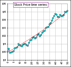

Figure 1 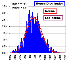Figure 2

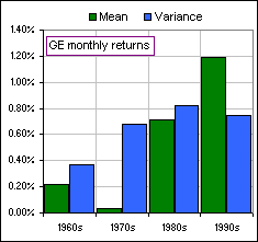Figure 3

>And the returns time series ... is it stationary? It would be if the distribution parameters (Mean, Variance etc.) are constant over time. >And are they? Are they constant over time? Look at Figure 3 where we note the Mean and Variance (that's StandardDeviation2) of the monthly returns for GE stock, over the 1960s, 1970s etc.. >I'd say non-stationary. Yes, me too.

Another thing we note (about how one often analyzes stock prices and/or returns) is the connection between two stocks in our portfolio.
It's customary to consider the correlation between the two returns series measured by R-squared / Pearson Correlation. Portfolio optimization and risk-reward analysis have usually been based upon correlation of returns, but a more recent consideration is the so-called cointegration.

>Huh?
When dealing with stock prices, it's been customary to first consider the difference between successive prices (and consider, instead, returns). This "differencing" eliminates any trends which may be involved and ...

>What's this cointegration stuff? Correlation is used to measure the ... uh, correlation between returns. When the returns for one stock go up or down, does the other tend to go up or down as well? It's a short term measure of interdependence. On the other hand, cointegration attempts to measure common trends in prices over the long haul. For example, suppose that the time series associated with two stock returns have a high correlation and the prices have high cointegration, as in Figure 4a. See the similarity in stock price trends? >Yeah, so? Okay, suppose we change the returns on one stock by a very small amount, replacing a return r by r - 0.001 (for example). The correlation between r and r - 0.001 is high. (Indeed, it's 100% !!) >But the stock prices are no longer cointegrated, eh? Yes, as in Figure 4b. >Okay, I know how to calculate correlation, but how do I calculate ...? How to calculate cointegration? That's what we'll talk about.

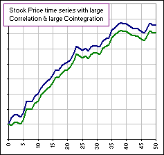Figure 4a 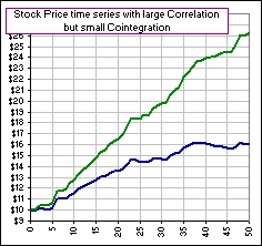Figure 4b

First, notice that if stock price (at time = n) increased according to Pn = P0 + r n + en where r is some growth rate and en is a random variable with Mean = 0 and Variance = v (and the correlation between pairs, such as en and en-m, is zero), then the mean of Pn would be P0 + r n (hence it's changing with the time, n) but the Variance would be constant at v (introduced by the random component en). >Huh? You can find the stat stuff here. Anyway, if you could identify "r" then the NEW variable Pn - (P0 + r n) would have constant Mean = 0 as well as constant Variance v. This NEW variable would be stationary, eh? In fact, from the relation Pn = P0 + r n + en we can see that Pn - Pn-1 = r + en - en-1 so this differencing has produced a stationary time series since en - en-1 has constant statistical parameters like: Mean = 0, Variance = 2v. >A stock price that increases in a straight line? I've never seen any ...?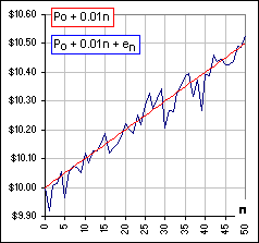

Figure 5

That's just an example. However, we might also be talking about spending habits where, as time progresses, we spend more and the national population expenditures might be considered to grow linearly ... with a random component. Or, the time series defined by P_n = P₀ + r n + e_n might be a relation between the logarithms of successive stock prices, like log[U_n] = log[U₀] + r n + e_n meaning that U_n = U₀e^{r n+e_n} implying a growth from some initial price of U₀ with annual (or monthly or daily) returns having a Mean equal to r.

Now let's consider a Random Walk where P_n = P_n-1 + e_n.

Then we'd have P₁ = P₀+ e₁ and P₂ = P₁+e₂ = P₀+e₁+e₂ and, eventually, P_n = P₀+e₁+e₂+ ... +e_n. Then the Variance is:
[1]     VAR[P_n] = VAR[e₁]+VAR[e₂]+ ... +VAR[e_n] = n v.

>That makes the Standard Deviation grow like SQRT(n), right?
Yes, the volatility would increase as time progressed ... becoming infinite.

Now consider a time series defined by P_n = ρ P_n-1 + e_n where, as before, e_n is a random variable with Mean = 0 and Variance = v.
Then P₁ = ρ P₀ + e₁, P₂ = ρ P₁ + e₂ = ρ² P₁ + ρ e₁ + e₂ and, eventually, P_n = ρⁿ P₀ + ρ^n-1 e₁ + ρ^n-2e₂ + ... + e_n.

Or, to put it differently:
P_n = e_n + ρe_n-1 + ρ²e_n-2 + ρ³e_n-3 + ...

Note that this expression defines the time series P_n as a moving average and ...

>Huh?
It's a sum with yesterday's e_n-1 having a weight of ρ and the day before having a weight of ρ² and the day before that having ...

>Yeah. So?
So the Mean of P_n is the sum of the means, which is zero, and the Variance is the sum of the variances (because the random components e_n, e_n-1, etc. have zero correlation) so Variance is:
[2]     VAR[P_n] = VAR[e_n]+VAR[ ρe_n-1]+VAR[ρ²e_n-2]+... = v+ρ²v + ρ⁴v + ρ⁶v + ... = v / (1 - ρ²)

>Where's P₀ and how did you get ...?
Okay, the fact that VAR[ρx] = ρ²VAR[e] is here and, uh ... we'll assume the time series is infinite and goes back forever.

>To simplify the math, eh?
Well ... yes, and it gives us a nice formula for the Variance since 1+ρ²+ρ⁴+ρ⁶+ ... = 1/(1 - ρ²).

>Okay, I'll stick in ρ = 10 and get ...
Uh, no, we can only write 1+ρ²+ρ⁴+ρ⁶+ ... = 1/(1 - ρ²)   if   -1 < ρ < 1.

However, if -1 < ρ < 1 then we can see from [2] that the Mean and Variance (and other stochastic parameters associated with P_n, like covariance) are constants so this time series is stationary. Of course, if ρ = 1 then we're in trouble.

>ρ = 1? Is that the unit root stuff?
Yes. In fact, the assumption that we started our time series in the infinite past gives rise to a stationary time series.
If we had started at some t = 0, we'd get a Variance which ended with ρ^2n-2e_n so depends upon n ... so it wouldn't be stationary.
Also, if had ρ > 1 it wouldn't be stationary.

Now consider two time series defined by:
[3A]     P_n = P₀ e^{r n} e_n
[3B]     P_n = P_n-1 e^r e_n

If e_n = 1, then [2A] and [2B] are the same. In fact, [3B] gives P_n = P₀ e^{r n} e₁e₂...e_n.

>That notation ... using "e" for the random component and for e^r ... you've done that before ... it's confusing!
Then concentrate!
Anyway, one may be tempted to say that there is little to choose between [3A] and [3B], however, we can write:
[3A.1]     log[P_n] = log[P₀] + r n + log[e_n]
[3B.1]     log[P_n] = log[P₀] + r n + log[e₁]+log[e₂]+...+log[e_n]

For the [3B] time series, there's a sum of random components (not just the current component, as in [3A]) and that makes the Variance grow with time, n.

>Is this stuff useful?
We'll see, but the point is that having a stationary time series is very handy. If, on the other hand, the Mean and/or Variance change from day to day, it's more awkward to do the statistical analysis. We'd like to see if some combination of the terms in the time series will result in a stationary time series.

>Like considering the returns instead of the prices?
Yes. Taking differences in successive prices or considering the percentage change ... that can eliminate trends as we saw in Figure 1.

>But calculating returns isn't the same as taking differences between successive prices ... is it?
Well, no. The returns involve a ratio:  P_n+1 / P_n. However, the difference between the logarithms gives log[P_n+1] - log[P_n] = log[P_n+1/ P_n].
The effect of differencing is to remove the trend (called, would-you-believe, "de-trending") and that may be bad as it removes the possibility of detecting common trends between two or more stocks. Nevertheless, it allows one to deal with a stationary time series. Imagine how one would determine the correlation between two time series if we dealt with prices or other non-stationary series. Now, using cointegration, one hopes to eliminate the need to calculate correlation coefficients yet identify common trends.

>Huh?
Suppose we wanted a portfolio of stocks chosen so as to "follow" the DOW. If we could arrange it so the tracking error (the difference between our portfolio and the DOW) was stationary, we'd be happy. It'd mean that our portfolio might deviate from the DOW but these deviations would have a Mean = 0 so portfolio values would oscillate about the DOW and ...

>Isn't that Mean Reversion?
Yes, if cointegration exists then there'd be mean reversion to the DOW index.

>Okay, so what IS cointegration? I mean ...
Two (or more) non-stationary time series are said to be cointegrated if a linear combination of the terms results in a stationary time series.
For example, if U_n and V_n are non-stationary but U_n - C V_n is stationary (for some constant C), then the two series are cointegrated (and there's an underlying, common trend). This would be the case if the "error", e_n = U_n - C V_n is stationary and therefore has time-independent statistical parameters: Mean, Variance and Autocovariance.

>Autocovariance?
Yes, the correlation between e_n and e_n-m, namely the Mean of (e_n - M)(e_n-m - M) ... where M is the Mean of the e_n.
This Mean can depend upon m (the "lag") but NOT upon n (the time). That (along with the time independence of the Mean and Variance) would make the time series e_n stationary. Note that, if m = 0, then the mean of (e_n - M)(e_n-m - M) = (e_n - M)² is just the Variance ... or (Standard Deviation)².