Once upon a time I played with the monthly returns for various world markets from Jan, 1975 to June, 1997 and found a number of interesting things I'd like to share (connected to the topic of Risk):

Did you know that:

1. There was not a single 2-year period when you would have lost money in the U.S. Large Cap market.
2. The chances of losing money in European Large Caps was only about 30% of the chance of making more than 10% ... over any 3-year period.
3. In Cdn Small Caps, you were 1 1/2 times more likely to make more than 10% annual return over any 12 month period than to make less than 0%.
4. In Pacific Large Caps, you would have lost more than 5% of your investment over a 6-month period 45% as many times as you would have made money.
   

Consider the following:
There are 246 intervals of length M=24 months (from Jan, 1975 to June, 1997).
You invest in Stock XYZ or perhaps Mutual Fund ABC.

• What fraction of these 246 24-month intervals would have given you an annual return greater than U = 10%? (U stands for Upper.) Suppose the answer is 0.5 meaning 50% these intervals would have given you an annual return greater than U = 10%).
• What fraction of these 246 24-month intervals would have given you an annual return of less than L = 0%? (L stands for Lower.) Suppose the answer is 0.1 meaning 10% of these intervals would have given you an annual return less than L = 0%.

The ratio gR³ = (fraction over 10%)/(fraction under 0%) = 0.5/0.1 = 5 means that you were 5 times more likely to achieve a return of 10% or greater than to make less than 0%.

>You could've just divided 50% by 10% and get 5, right?
Uh ... yes.

>What if gR³ = 2?
Twice as likely to achieve 10% than to lose money.

In fact, for Canadian Large Caps, we have gR³ = 2.0 and for other markets we have the following values of gR³:

Cdn Large Cap 2.0
Cdn Small Cap 1.5
U.S. Large Cap 4.9
U.S. Small Cap 7.6
Euro Large Cap 3.2
Asia Large Cap 1.7

Of course, gR³ depends upon the values of Months, Upper and Lower (as well as the total time interval Jan/75 - Jun/97, of course). We'll call it gR³(M,U,L), so that, since the above list considered the case M = 24 months and more than U = 10% and less than L = 0%, then we're talking about gR³(24,10,0).

From the above list we can see that for US Small Caps, gR³(24,10,0) = 7.6 meaning you were 7.6 times more likely to achieve 10% annual return than to lose money, over any 24 month period!

If you've come this far along, you may be interested to know that:

1. gR³(24,0,0) = infinity for the U.S. Large Cap market.
2. gR³(36,10,0) = 3.3 in European Large Caps.
3. gR³(12,10,0) = 1.5 in Cdn Small Caps.
4. gR³(6,0,-5) = 2.2 in Pacific Large Caps.

>Why gR³ ? Why not gR², like E = m c² ?

For those gallant few who have made it this far, R³ stands for Reward Risk Ratio:

making LESS than L = 0% is the Risk and making MORE than U = 10% is the Reward and we consider the Ratio      so far, we've got R3

... and can y'all guess what g stands for?

>The Market Data, can we trust it? Where'd it come from?
Uh ... the data for the various large/small cap markets was obtained here:

>Where's the pictures? You usually have pictures! I mean ...
Here's one:
We consider all the N-year periods starting each month from Jan, 1928 to Year 2000. Then all the N-year periods starting in Feb, 1928 then starting in Mar, 1928 etc. etc. and determine the percentage where the annualized gain exceeded 10% and compare it to the percentage where the gain was less than 4%. The ratio would be ...

>Don't tell me! It's gR³(360,10,4) ... for 360 months and 10% and 4%, right?
Very good, but 360 would be for 30 years. In general ... well, here's the picture:

>Uh ... does that mean that, over 25 years, 68% of annualized returns were greater than 10% and ...
And none were less than 4%.
>That makes 25 x 12 = 300 months so gR³(300,10,4) = 68/0 = ... uh ...
Infinite. However, one can judge what the "risk" might be for various asset allocations just by staring raptly at the chart. For example, here's a similar chart where, instead of just the S&P 500, we invest in a 4 x 25 portfolio: 25% in each of Large/Small Cap and Large/Small Value and rebalance yearly.

However, if we're lookimg for a single number which (somehow!) describes "risk" ...

Suppose we look at the monthly gains (for some stock or mutual fund) which are greater than some pre-assigned percentage, U (meaning Upper), and those which are less than some pre-assigned percentage, L (meaning Lower).

We'll label the set greater than U like so:	u1, u2, u3 ... uN
and those less than L like so:	l1, l2, l3 ... lM

assuming there are N of the former and M of the latter. We're using the subscript "k" to denote a particular member of the set, so k = 1 or k = 2 or ...

Uh ... let's assume we ALWAYS choose L = 0 so the L-set corresponds to NEGATIVE monthly gains - that's the risk, right? We also choose U > 0 so it corresponds to POSITIVE monthly gains. Our goal is to invest so that the U-set is huge and the L-set is microscopic.

It's a battle.

Will the u's win?
Will the l's win?

GO U-set!!

In particular, if we plot the distribution of monthly gains for the S&P 500 we get the chart at the right (for the period Jan, 1970 to Jan, 2000) which gives the number of monthly gains in each interval. >Finally! A picture! A picture is worth a thousand - Okay! Pay attention! Notice that's the distribution is close to being Normal ... the infamous Bell Curve. Later we may just assume it is normal. In the meantime, we want to ignore those gains which lie in the interval L < gain < U because we're only looking at the gains to the left of L = 0 or to the right of U = something_positive.

Fig. 1

Fig. 2

If we delete that part of the chart we get the chart at the left where, for the sake of concreteness, we've assumed U = 4% and, of course, L = ... >Concrete? Did you say - Now we throw darts at the chart ... >Darts? Did you say - ... and see if it hits the L-set or the U-set. If it misses either of these, we ignore the dart toss. Then we see what percentage of our dart throws (not counting those which miss everything) result in a GOOD gain, lying in the U-set, compared to those which result in a BAD gain.

The percentage is the Area of the U-set divided by the Area of the L-set. For the case shown above, it's 1.08

Our conclusion? During the period Jan/70 to Jan/00, you were just slightly more likely to make a monthly gain more than 4% than you were of losing money.

>That's pretty lousy! Of course, but asking for a monthly gain exceeding 4% is rather optimistic. If we ask only that it's greater than 1% (that's about 12% per year), then the ratio is about 2. We were twice as likely to make a monthly gain exceeding 1% than making a negative gain. >Picture! Picture!     Okay, here's a little picture of the L and U distribution(s)     >So I'd be twice as likely to make 12% as losing -

Fig. 3

We were talking about a single month here! Any of the 360 months in that thirty year period. Of course, we could also talk about the 12-month gains or the 24-month gains or ... >So this ratio depends upon U and L and M ... sounds familiar. Right. Now let's simplify the prescription for computing this ratio. Here's what we'll do: Determine the Mean and Standard Deviation of the monthly returns. Assume they are normally distributed, and construct a normal curve with the same Mean and SD. Delete the portion between L and U           like so Compute the ratio of Areas, using well-known formulas ...

Fig. 4

>Well known? You're kidding, right?
Pay attention.
Let's assume that L = 0 so that the L-set corresponds to investment losses. In any case, that's what Fig. 4 illustrates. Oh, and I should mention that the vertical axis, in Fig. 4, doesn't measure the NUMBER of returns but the FRACTION of returns. Earlier, in Fig. 1, if we computed the total Area we'd get the total NUMBER of monthly returns, namely 360 (in the thirty year period). Here, in Fig. 4, the total Area would be "1".

>That's confusing ...
Okay, we just take all the numbers along the vertical axis in Fig. 3 and divide them by 360 and we'll get a fraction and that gives us Fig. 4 which we've also smoothed out so it's a normal curve.

Now, suppose we have a magic formula for the area, from x = a to x = b, under a normal curve which has Mean = m and SD = s. We'll call it A(a,b,m,s). Stare at Fig. 5 to see the area we're talking about. Then our Risk Ratio is : A(U,∞,m,s) / A(-∞,0,m, s) Remember, the TOTAL area under the curve is "1", so A(-∞,∞,m,s) = 1 and if we choose U = the Mean monthly gain, then A(m,∞,m,s) = 0.5 >... and the magic formula for the area?

Fig. 5

Okay, let's do it. If y'all hate calculus, you can skip this part and go here.
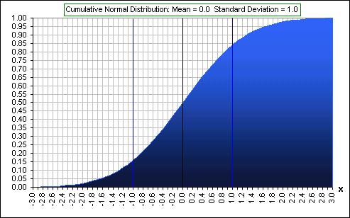
The Normal distribution (meaning the equation of the normal curve, most of which is shown in Fig. 5) is

We'll call this function f(x,m,s) and the magic formula for the area A(a,b,m,s) is:

Whereas there are tables of areas for normal distributions with Mean = m = 0 and SD = s = 1, there ain't hardly none for arbitrary Mean and SD ... so we transform our function like so:

Set x = m + s t in the distribution function f(x,m,s) and get     f(x,m,s) dx = f(t,0,1) dt
and we've succeeded in transforming to Mean = m = 0 and SD = s = 1.

The limits "a" and "b" also change to (a - m)/s and (b - m)/s. In particular, our Area function becomes:

A ( a,b,m,s) = A ((a - m)/s ,(b - m)/s,0,1 )

So where are we?

1. We determine the Mean m and Standard Deviation s of the historical monthly returns.
2. We assume they are normally distributed.
3. We select some U value (making it a fraction, so 1.2% means U = .012 and we assume L = 0 so that "risk" is a risk of losing).
4. We compute the ratio A(U,∞,m,s) / A(-∞,0,m, s) , namely:

A ((U - m)/s ,∞)) / A (-∞ ,- m/s)

where A (p,q) is the probability that a variable (normally distributed with Mean = 0 and SD = 1) lies between p and q.

> ... zzzzzz ...
Well?
>Uh ... where's the root of s?
It's a factor of both numerator and denominator so it cancels out. Neat, eh?

> ... zzzzzz ...

---

Okay, here's a picture of the cumulative normal distribution A(-∞,x) (the Area function we talked about earlier, where we consider EVERYTHING less than a value "x") with Mean = 0 and Standard Deviation = 1:

Fig. 6 Cumulative Normal Distribution, showing the fraction of values less than a given value

I've drawn a vertical line at x = -1. That's one Standard Deviation below the Mean of 0. Reading off the chart, a normally distributed random variable will have 0.16 of its values less than -1. There's a second vertical line one SD above the Mean, at x = 1 and, again, reading off the chart, 0.84 of the values will be less than +1. We conclude that 0.84 - 0.16 = 0.68 of the values of a normally distributed random variable will lie between x = -1 and x = 1. That is, 68% will lie within one Standard Deviation of the Mean.

>As long as the Mean is zero and the SD is ...
Well, actually, it's true for any Mean and SD. If we increase (or decrease) the Mean by some amount, the chart just slides to the right (or left) by that amount. If we increase (or decrease) the SD by some amount, the chart expands (or contracts) horizontally.

>Contracts horizontally? Here's a picture to illustrate, where we decrease the Standard Deviation from SD = 1 to SD = 0.5 and you can see that it contracts ... horizontally, eh? The two values at x=-SD and x=+SD, namely 0.16 and 0.84, are the same so their difference still gives .68 or, to use the standard recitation of investment gurus: "2/3 of returns lie within one Standard Deviation of the Mean". >But 68% isn't 2/3. It's close enough. >Is this measure of risk any good? Well, let's put it to the test.

Cumulative Normal Distribution, showing the effect of changing the SD

We'll consider the monthly gains for the stock General Electric from Jan, 1970 to Jan, 2000 ... 360 months, where we get the data here.

• The average gain was 1.3% (so we put Mean = m =.013)
• The Standard Deviation was 6.5% (so we put SD = s = .065).
• We'll select our "reward" as 1% (meaning any monthly gain of 1% or more is a GOOD gain). That puts U = .01, so
• we now compute (as prescribed above) the number (U - m)/s = (.01 - .013)/.065 = -0.046
  and the number - m/s = -.013/.065 = -0.20
• Now we compute (as prescribed above) the Ratio:
  A ((U - m)/s ,∞)) / A (-∞ ,- m/s) = A(-0.046,∞) / A(-∞,-0.20)

>Wait! What's this (1 - 0.48) stuff?
We get, from Fig. 6, that the fraction of values which are less than -.046 is 0.48, hence the fraction above -.046 is (1 - 0.48). Anyway, we conclude that you were 1.23 times as likely to have a monthly gain greater than 1% than you were to lose money, in GE stock, over the thirty years 1970 - 2000. That's 23% more often. That's good, isn't it?

>But you already have the data. Is it true? I mean that percentage, 23% ... was it 23%?
Hmmm, good question. Let's see ... I'm looking at the data ... there were 178 months with gains of 1% or more ... and 160 with negative gains ... that gives a Ratio of 178/160 = 1.11 so ...

>Aha! Just as I thought! You're way off the mark! A wise man once said:

---

Here's another neat thing. A measure of Risk which goes like so: We assume a set of Returns with a certain Mean and Standard Deviation. We assume they're distributed Normally. We determine, from the Normal Cumulative Distribution, the percentage of Returns which are negative. It'll depend upon the ratio Mean/SD We define that percentage as the Risk. It looks like so: See also another Frontier.

In any case, let the gurus use their silly definitions, like "Volatility = Risk".
For us mere mortals, let us not say that the GREEN stock
has been a riskier investment than the RED:

Let's just say it's been more Volatile.

Here's another definition of "Risk":

>Is it any good?

Okay, here's the question:

Over the past umpteen years, investment A has had a Mean return of 10% and a Volatility of 20%.
Investment B has had a Mean return of 12% and a Volatility of 25%.
Investment B has had a higher Volatility ... hence has been more risky.

Now suppose there existed a (fictitious) Mutual Fund which guaranteed a minimum annual return.
The chart looks like so, for the past twenty years.

The Volatility has been greater than the S&P 500 ... so it's riskier.

>Do you believe that?

Several Nobel prize winning physicists DEFINE "Green Cheese" to mean the constituents of the moon.
The headlines read: "The moon is made of Green Cheese!"

Ain't definitions wunnerful?
You can turn the moon into green cheese
... and Volatility into Risk