First, some items :

1. If a stock first increases by 13%, then decreases by 13%, it will not return to the original stock price,
   since (1+0.13)(1-0.13)= 0.9831 so the stock returns to just 98.31% of its original value.
   In order to return to the original price an increase by a factor (1+0.13) must be followed by
   a decrease by a factor 1/(1+0.13) ... then, when you multiply, you get "1".
2. Some mathematical notes:
   (x+y)² = x² + 2 xy + y²     with binomial coefficients 1,2,1
   (x+y)³ = x³ + 3 x²y + 3 xy²+ y³     with binomial coefficients 1,3,3,1
   (x+y)⁴ = x⁴ + 4 x³y + 6 x²y²+ 4 xy³ + y⁴     with binomial coefficients 1,4,6,4,1
   (x+y)⁵ = x⁵ + 5 x⁴y + 10 x³y²+ 10 x²y³ + 5 xy⁴ + y⁵     with binomial coefficients 1,5,10,10,5,1
   etc. etc.
   hence the magic formula
   (x+y)^N = N₀x^N + N₁x^N-1y + N₂ x^N-2y²+ ... + N_Ny^N       where the binomial coefficients are
   or, equivalently:
   (x+y)^N = N_Nx^N + N_N-1x^N-1y + N_N-2 x^N-2y²+ ... + N₀y^N
   or, equivalently:
   (1+x)^N = N₀ + N₁ x + N₂ x² + ... + N_Nx^N

>Those binomial numbers ... aren't they usually called _NC_m or ?
Yes, but it's too cumbersome for me to write, so just remember this N_m notation, okay?
>Do I have to know all this?
Pay attention ... and don't interrupt again.

We follow the movements of a stock over successive days (or hours or months or whatever). We assume that, if its current price is S, then it will do one of two things: it will change by a factor U = 1+g, taking on the value US (if it goes Up) or it will change by a factor D = 1/(1+g), taking on the value DS (if it goes Down) after N Ups and M Downs it will have the value UNDMS all stock prices, after N ups and M downs, are possible (though with different probabilities) the diagram illustrates the case where the stock price has changed 5 times and a particular stock-price-path has been identified (in magenta). In how many ways can a particular stock price be attained? 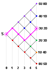For example, how many stock-price-paths lead to the price U3D2S (namely 3 Up and 2 Down), after 5 time periods?

Figure 1

• 5 Up and 0 Down is 5₀ or 5₅, namely 1
• 4 Up and 1 Down is 5₁ or 5₄, namely 5
• 3 Up and 2 Down is 5₂ or 5₃, namely 10
• 2 Up and 3 Down is 5₃ or 5₂, namely 10
• 1 Up and 4 Down is 5₄ or 5₁, namely 5
• 0 Up and 5 Down is 5₅ or 5₀, namely 1

So what's the probability p?
>You said I shouldn't interrupt.

First we note that investors are less likely to drive up the price of a stock if it's gain is very much greater than the risk free rate. In fact, the higher the Up gain factor, U (relative to the risk-free gain factor R), the smaller the probability of achieving this Up-gain. To mathematize this notion, we set the probability of achieving the Up factor as p = (R - D) / (U - D) as indicated

Figure 2

>The risk-free gain factor?
Yes. If, for each time step, the risk-free return is r (where r = 0.012 means 1.2%), then R = 1 + r is the risk-free gain factor.
Okay, we now attach a probability to each final state of the stock price, after n Ups and m Downs.
Since each of the n Ups has a probability of p and each of the m Downs has a probability of 1-p, I think it's clear that
      the probability of n Ups and m Downs is pⁿ(1-p)^m
>Clear? To who?
To whom. Just be quiet and pay attention.

Note something interesting.
After N time steps, the probability of achieving at least one of the terminal stock values must be 1.
>Meaning 100%, eh?
Yes. This probability is just the sum of the individual probabilities, namely the sum of things which look like:
      (Number of ways to achieve a given stock price)x(Probability of achieving that stock price)
namely:
      N₀p^N+N₁p^N-1(1-p)+ N₂p^N-2(1-p)²+ N₃p^N-3(1-p)³+ ... + N_N(1-p)^N
>Are you saying that's equal to 100%?
No, I'm saying it's equal to 1 because, according to the magic formula in item 2 above (with x replaced by p
and y replaced by 1-p):
{p + (1-p)}^N = N₀p^N + N₁p^N-1(1-p) + N₂ p^N-2(1-p)²+ ... + N_N(1-p)^N
and, of course, {p + (1-p)}^N = 1^N = 1.

We can write this like so:

(*)       {p + (1-p)}^N = Σ p^N-m (1-p)^m = 1     or, equvalently     Σ p^m (1-p)^N-m = 1

>So there are lots of possible stock prices, right?
Yes, and each has an associated probability. However, the "Expected Value" of the price is a sum of things which look like:
      (Probability of achieving a particular price)x(the price)
namely:
      N_Np^N [U^ND⁰S] + N_N-1p^N-1(1-p) [U^N-1D¹S] + N_N-2p^N-2(1-p)²[U^N-2D²S] + ... + N₀(1-p)^N[U⁰D^NS]
where we now know the associated probabilities and we've again used the magic formula in item 2, above.

We'll rewrite this formula using a more familiar notation for the binomial coefficients:

(1)     Expected Stock Price = Σ pm(1-p)N-m UmDN-mS = S { p U + (1-p)D }N

We assume it's worth $C today and $E after N steps. If we invested our $C at the risk-free rate (meaning a gain factor of R per time step) it would grow (after N time steps) to C R^N which, if we want to assume no risk, should equal the expected price of E.
Hence C R^N = E so C = E R^-N.
In other words, the current value of the stock should be the expected value, after N steps, divided by R^N.
In other words, we're discounting the end-value to the current-value by discounting at the risk-free rate.
In other words ...
>That's enough other words.

Okay, we'll write as and divide by R^N which we'll split up as R^mR^N-m and rearrange/combine stuff to get:

(2a)     Current Stock Price = S Σ {pU/R}m{(1-p)D/R}N-m

Do you recognize this expression?
>Are you kidding?
I mean, its form. The way it looks. Is it familiar?
>Are you kidding?

Notice that there are two curious factors in this summation, namely P = {pU/R} and {(1-p)D/R}.
The first of these can be rewritten as P = {(R-D)U}/{R(U-D)}, since p = (R-D)/(U-D) ... see figure 2.
Further, 1 - P = 1-{(R-D)U}/{R(U-D)} = {(U-R)D}/{U-D)R} = {(1-p)D/R} which is the second curious factor.

Hence, we can rewrite the formula above as:

(2b)     Current Stock Price = S Σ {P}m{1-P}N-m where p = (R-D) / (U-D) and P = pU/R

Okay, now for a revelation!

Look again at formula (1), above, namely:
(1)     Expected Stock Price = S { p U + (1-p)D }^N   where p = (R - D)/(U - D)

Look carefully at p U + (1-p)D = p (U - D) + D = {(R - D)/(U - D)} (U - D) + D = {R - D} + D = R

In other words, if we assume that the probability of an Up is p = (R - D)/(U - D)
then we're expecting our stock to grow at the Risk-free rate!!

Okay, we now look at formula (2b), above, namely:
(2b)     Current Stock Price = S Σ {P}^m{1-P}^N-m

But, according to our formula (*) above, this can be rewritten:
(2b)     Current Stock Price = S {P + (1-P)}^N = S

>Isn't that obvious? I mean, we already assumed we started with a stock whose price is S, so ...
So why didn't pick that out?

>So all the stuff above is garbage, eh?
No. It just means that picking the Up probability as (R - D)/(U - D) is equivalent to assuming we'll get just the Risk-free growth. We can choose ANY value for p, right? In fact, if we choose an arbitrary p, we're ignoring the Risk-free Rate. Besides, the various manipulations we did above were quite edifying, right?

>Wrong! Do you realize that you hardly have any pictures?

Figure 3

They are Binomial Probability functions: f(m) = density and F(m) = cumulative.
Have you seen them before?
>Never!
Looks much like the standard Normal distributions, eh? Especially for the larger N.

The binomial distribution, defined by B(N,m,p) = p^m(1-p)^N-m, is your basic, all-purpose probability distribution.
Actually, binomial probabilities describe a process where there are just two mutually exclusive outcomes, each having an associated probability (namely p and 1-p). Tossing a coin would have p and 1-p both equal to 0.5 and, if we had a pair of dice, each having ten sides, and six of the sides said UP and four said DOWN then, throwing a single die would have ...
>Don't tell me! 60% chance of UP and 40% chance of DOWN.
Yes, so p = 0.6 and q = 0.4 and ...
>So, what's the Mean and Standard Deviation? For a Normal distribution they define the distribution, right?
Yes, they do ... so we'll find them for the Binomial distribution:

B(N,m,p) = p^mq^N-m

Note that this is the probability of getting a value m out of N trials.
>Like getting m heads out of N tosses of a coin?
Exactly. If we call this probability P(m), then the Average (or Mean or "Expected") value is a sum of things which look like:
      (the value m) x (Probability of achieving the value m) = SUM[m P(m)], namely
            Mean = Σ m p^mq^N-m     where the sum goes from m = 0 to m = N

however, the first m = 0 term has the value 0, so we might as well start at m = 1.

Now we go through the following ritual:

[ritual 1]            

and now we let k = m-1 so k goes from 0 to N-1 and we get (after factoring out Np):

            Mean = Np Σ p^kq^(N-1)-k     where the sum goes from k = 0 to k = N-1

and now we stare at item 2 again and recognize:

            1 = 1^N-1 = [p + (1-p)]^N-1 = Σ p^kq^(N-1)-k     where the sum goes from k = 0 to k = N-1

so, finally (!) we conclude that:

           

Mean(of the Binomial Distribution) = Np

>In Figure 3 the means are 0.6 x 15 = 9 and 0.6 x 100 = 60, right?
You got it.
>And the Standard Deviation?
The Variance (the square of the Standard Deviation) is obtained from a sum of terms which look like:
      (Deviation of m from its mean Np)²x(Probability of getting the value m)

namely:
            SD² = Σ (m - Np)² p^mq^N-m     where the sum goes from m = 0 to m = N

>Let's just skip that one ...
It's not that bad. In SD stuff we showed that SD² = (Average of the Squares) - (Square of the Average) so:

            SD² = Σ m² p^mq^N-m - (Np)²

Now we go through a second ritual (using the first ritual, above):

[ritual 2]            

which enables us to rewrite the above expression as:

            SD² = N(N-1)p²Σ p^m-2q^(N-2)-(m-2) + NpΣ p^m-1q^(N-1)-(m-1) - (Np)²

and each sum equals "1" (as per item 2) so we get (finally!):

            SD² = N(N-1)p² + Np - (Np)² = Np(1-p) = Npq

Hence            

Standard Deviation(of the Binomial Distribution) =

>So, in Figure 3, the standard deviations are 15 x 0.6 x 0.4 = 3.6 and 100 x 0.6 x 0.4 = 24, right?
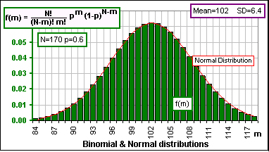
Actually, the square root of those numbers, namely SQRT(3.6) = 1.9 and SQRT(24) = 4.9 but, in any case, our goal is to see what happens when N is large. To this end, we show the Binomial and Normal distributions with the same Mean and Standard Deviation, like so:

>But if you let N get larger and larger then the Mean and SD also become ...
Larger and larger? You're quite right, but we can avoid that by shifting the curves to the left (so the Mean is 0) and scaling ...

Let's do the following:

We'll assume an Historical Annual Return of 9%
    hence an "equivalent" monthly rate of 9/12 = 3/4% so g = 0.0075   ... an historical monthly return
    so U = 1 + g = 1.0075 and D = 1/U = 0.99256 (giving the UP and DOWN monthly gain factors)
    and we'll assume p = 0.70     ... implying that our stock goes UP 70% of the time

>This is fiction, right? Up, 70% of the time? And what's with that "equivalent" monthly gain ...?
Pay attention. We're playing a game here. Later, I'll give you a calculator which doesn't bother with the "equivalent" monthly returns.

Continuing:
We'll flip a coin - a coin which comes UP (meaning we get a Heads) 70% of the time in which case our stock price increases by the factor
U = 1.0075 and, if it comes up Tails (that's a DOWN), the stock price changes by a factor D = 0.99256 (that's a monthly loss, eh?) - and we do this flipping each month for umpteen months ... and we use that binomial stuff to see what the distribution of stock prices would be after a year or three and calculate an Expected Stock Price and ...

>A picture would be good.
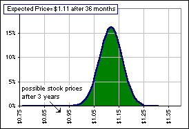
Here's a picture, with an initial Stock Price of $1.00:

>What's that horizontal axis?
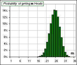
That's m, the number of UPs.
For example, for a 3 year scenario (meaning 36 monthly coin flips) the most probable number of UPs is 25 of them ...
>That's the formula: N p = 36 (0.70), right?
Yes, and if we associate a probability with a stock price we can calculate an Average or Expected Stock Price and that's shown on the chart.

>I still find it confusing. I mean ...
Okay, consider the case 36 months:

The total number of possible UP/DOWN sequences is 236 The number of times m heads occurs (in this set of possibilities) is ... with N = 36, for our example. Figure 4a shows the percentage of these possibilities which give m UPs. (Note that about 13% of the 236 possible UP/DOWN sequences have m = 18, as shown in red in Figure 4a.) Aah, but the probability of getting m = 18 UPs is NOT 13% since we aren't tossing a "fair" coin; our coin comes up Heads 70% of the time! In fact, the probability of getting m UPs is pm(1-p)N-m which, for our example (where p = 0.70 and N = 36) is largest for m = 25, as seen if Figure 4b. Further, not only are we likely to get lots of Heads, but our stock price goes UP by a factor of 1.0075 each time a Heads occurs and we then consider all possible sequences of Heads/Tails (or UPs/DOWNs), each with its attached probability. (We could get a jillion heads, but if they aren't associated with any gain, our expected stock price wouldn't be too exciting, eh?). Anyway, we get Figure 4c: Figure 4c

Figure 4a Figure 4b

Note: Using a formula we obtained above, we have (for our example):

    Expected Price = { p U + (1-p)D }^N = { (0.70)(1.0085) + (1-0.70)(0.99256) }³⁶ = $1.11

Here's a calculator to play with. Note that it assumes we start with a stock worth $10, not $1.
It also ignores that "equivalent" monthly return and uses the annual returns directly (which explains why the answer is slightly different than the example considered above). Note, too, that the return g is actually an estimation of the gain when the portfolio goes UP !!
(It should therefore be chosen somewhat larger than a historical annual return.)

Using:   Expected Stock Price = S { p U + (1-p)D }N with S = $10   and U = 1 + g,   D = 1/U

Assumed Annual Stock Return g = %     when the stock goes UP! Assumed Risk-free Return r = %     which won't affect the answer below! Probability of a Gain p = % Number of Years N = Expected Stock Price = $     after N years

>Calculators are nice, but pictures are better!
Here's a simple spreadsheet which gives pictures

Just RIGHT-click on the picture of the spreadsheet and Save Target.

See also tossing coins