It has been said that the distribution of monthly (daily? yearly?) returns are Normally distributed. That is, the frequency with which certain returns occur lie on a "Normal" curve. We want to understand what this means and to determine whether such an assumption is valid or simply a mechanism for applying some esoteric mathematical ritual. A wise man once said: "What faith one should place in the conclusions drawn from such assumptions is a religious argument."

First we consider 600 numbers (which we'll express as a percentage because we'll eventually be considering monthly percentage gains in the S&P 500 index). We suppose these percentages all lie between -12% and +14%. Here's what we'll do:

We count the number of percentages less than -12%: 0 We count the number of percentages less than -10%: 2 We count the number of percentages less than -8%: 7 We count the number of percentages less than -6%: 25 etc. etc. We count the number of percentages less than +14%: 600 Now we plot the points (-12,0), (-10,2), (-8,7), etc., (+14,600) and we get Fig. 1 (where we've also drawn a smoooth curve joining these points - indicated by wee red squares). The Average (or Mean) of the 600 percentages is 1%, in this example, and half of the 600 (that's 300) are less than the Mean. This is the Cumulative distribution for our 600 percentages (and, for this example, we've actually plotted a Normal Cumulative distribution - so we can see what it looks like).

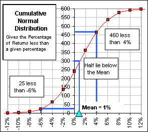Fig. 1

Now let's consider the number of these 600 percentages which lie in the intervals: (-12% to -10%)   (-10% to -8%)   (-8% to -6%)   ... (+12% to +14%) We can actually get these numbers from Fig. 1. For example, if 460 are less than 4% and 355 are less than 2%, then 460 - 355 = 105 lie between 2% and 4%. We then plot a point at 3% (half-way between 2% and 4%) and give it the value 105. That's one point in our graph (shown in blue). The points, complete with smoooth curve, are shown in Fig. 2 This is the familiar (infamous?) Bell Curve and gives the Density distribution for our 600 percentages. Note: If we count the number in (-12 to -10) and those in (-10,-8) etc. and add all these numbers we get ... 600!

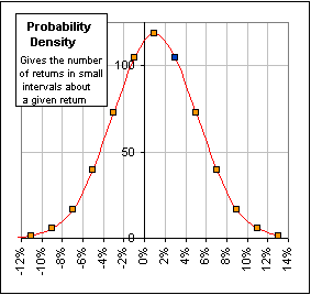Fig. 2

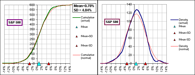
Fig. 3a         and         Fig. 3b

In each case there's a thin red curve which is an actual, real, live Normal Curve (as opposed to the distribution of S&P 500 returns). Stare at Fig. 3 for a while and one starts to believe that these monthly returns are, indeed, normally distributed.

>Are you kidding? The Density guy is way off! Isn't there some better fit? Some theoretical distribution which gives a better match? One that ...?
Uh ... there's also a Log-normal distribution which is quite popular among analysts. Before we get to that, however, let's look more carefully at the Normal distribution.

If we consider the range of returns from Mean - Standard Deviation to Mean + Standard Deviation, the real live Normal distribution will have 68% lying in that interval. (See SD stuff.) For the S&P500, the mean monthly return is 0.78% and the SD is 4.04% so the range is from 0.78 - 4.04 = -3.3% to 0.78 + 4.04 = 4.8% and, as it turns out, 73% of the monthly returns for the S&P lie in that interval. Actually, you can sorta see that from Fig. 3b where the returns are more closely scrunched near their Mean, compared to the red, Normal distribution.

>Scrunched? Is that a technical term?
Further, the range of monthly returns is from -100% to + infinity (meaning unlimited upside gains) whereas the Normal density function expects a range from - infinity to + infinity.

>Is that bad?
Not bad. It just means that assuming a Normal distribution for the S&P is just an approximation, and approximations are just ... uh ... approximations.

Let's move on to the Log-normal distribution.
>Wait! What info do I need to plot a Normal graph? Do I need hundreds of points or ...?
Actually, you just need the Mean and Standard Deviation of the distribution and, armed with these two numbers, the Normal distribution is defined.

Let's move on to the Log-normal distribution. To understand it we do a bit of math ...

>Do we have to?

1. Let r₁, r₂, ... r_N denote N monthly returns     where r = 0.0123 corresponds to a monthly return of 1.23%
2. Assume that -1 < r_n < infinity     assuming that no month will reduce our investment to zero ... or less!
3. Let g₁, g₂, ... g_N denote the monthly Gain Factors     where g_n = 1 + r_n
4. Then 0 < g_n = 1 + r_n < infinity
5. Then -infinity < log(g_n) < infinity     so the logs have the appropriate range for a Normal distribution!
6. Consider the distribution of the N logarithms, x_n = log(g_n)
7. Assume that the x_n are Normally Distributed.
8. Then we say that the g_n have a Log-normal distribution.

>That's confusing
If the set of logarithms, log(g_n), are Normally Distributed, then we say that the set g_n has a Log-normal distribution.
In other words:
If a set {g} has a Log-normal distribution, then it means that g = e^x where the set {x} has a Normal distribution.

>You forgot your subscripts.
Let me leave them out - for sanitary reasons.
So instead of saying g₁, g₂, ... g_N I'll just say {g} and instead of saying g_n=1+r_n I'll just say g=1+r and instead of ...
>Okay, I get the idea. And what about the S&P500?

Okay. Here's what I did:

• I looked at all six hundred monthly returns, {r} expressed as a decimal, like 0.0123, instead of a percentage, like 1.23%
• then the monthly Gain Factors {g} = {1+r}
• then their logarithms {log(g)} the natural log, to the base e, tho' that isn't important
• then calculated the Mean and Standard Deviation of these 600 logs
• then I plotted the Cumulative and Density distributions for these 600 logs as described above
• and I compared them to a real, live Normal distribution with the same Mean and Standard Deviation
  cuz if these Gain Factors had a Log-normal distribution, their logs should have a Normal distribution
• and I got:

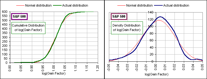
Fig. 4a         and         Fig. 4b

>That's pretty lousy, and besides, plotting against a logarithm seems sort of ...
Okay, here's a picture of a Log-normal and a Normal distribution, having nothing to do with the S&P500; just an example (plotting the percentage of values, unlike Fig. 4 which plots the number) to show how the Log-normal Density distribution is skewed to the right with a fatter tail - that's kurtosis - whereas the Normal distribution is nicely distributed about the mean which, in this example, happens to be 3.0.

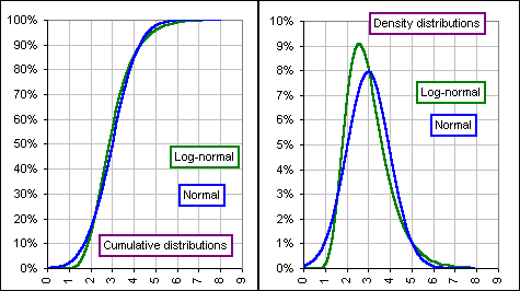
Fig. 5a         and         Fig. 5b

>Kurtosis? My doctor said ...
One neat thing about considering the logs ...

>Wait! You said the Mean for Fig. 5 was 3.0 yet the Log-normal curve lies mostly below the mean - I mean to the left of the mean - but only half of the points, that's 50% of 'em, should lie below the mean, right? Wrong. For the Log-normal distribution, more than 50% lie below the mean because of the skewness ... >Is that possible? The four numbers 4, 4, 4 and 100 have a mean of 28, yet more than half of these numbers are below the mean. In fact, 3/4 of them are below their mean.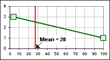

Anyway, one neat thing about considering the logs of the monthly ...
>Wait! What about the S&P500 monthly gains?
Uh ... 48% of the six hundred monthly gains are less than their mean ... which is 0.78%.

Anyway, one neat thing about considering the logs of the monthly gain factors (instead of the gain factors themselves) is that $1.00 invested in the S&P500 grows to g₁ after one month, then g₁g₂ after two months, etc. and g₁g₂...g_N after N months and, since g=e^x where x = log(g), we get the neat result:

Note:
Here's something interesting.

• The Gain Factor for a single year is then e^(1/N)Σx = e
  where Mean[x] = is the average or Mean of the x's.
• The Annualized Gain is then e - 1.
• If the x's are normally distributed, then 50% of them are above Mean[x] and 50% below.
• Hence 50% of the Annualized Gains are above and 50% below e - 1.
• The Median Annualized Gain is then e - 1.

>You forgot your subscripts.
Pay attention. The set of numbers {x} = x₁, x₂, x₃ ...

>I was going to ask about them. What are they? ... are very nearly the actual monthly returns: r1, r2 etc. That's because g=1+r is close to 1 (unless the monthly gain is huge) and since g=ex it means that x is close to zero and that means that ex is very nearly equal to 1 + x ... see the graph of y = ex and y = 1+x so that means ... >Don't tell me! g = 1+r and g = 1+x, nearly. So x = r, nearly. You got it.

>Hold on! We don't like assuming that the monthly returns, r, are Normally distributed so we turn to a Log-normal distribution where we assume that the set {x} is Normally distributed and then find that x = r, very nearly, so is the analysis so precise that ... ?
Good question! I suspect that, as much as anything, it's the neat mathematics that follows from a Log-normal distribution that prompts people to assume Log-normal. Let me explain:

>Hold on! If Log-normal assumes that log(g) is Normally distributed then I assume that the number lying within one standard deviation of their mean is closer to 68%, like the real, live Normal ...
Good point. Actually, 73% of the six hundred log(g) values lie within one Standard Deviation of their Mean, so ...

>But that's the same as the plain Jane Normal, right?
Actually, for the gains themselves, to one decimal place, it's 72.7% and for their logs it's 73.2% so ...

>So, assuming that the gains are Normal is better than assuming they're Log-normal, right?
Well ... uh ... if the 68% is your only goal in life and the S&P your only investment and those fifty years from 1950 to 1999 your only time period, but there are other things to consider.

>Like what?
Okay, but first we should identify certain properties of both Normal and Log-normal distributions.

1. If a and b are constants, then the set {a + bx} is N(a+bμ,b²σ²)   ... it has Mean=a+bμ, Variance=b²σ²
2. {y} is a Log-normal distribution if y = EXP(x) where {x} is Normal: N(μ,σ²).
3. The Mean of {y} = {EXP(x)} is EXP(μ+σ²/2) and its Variance is EXP(2μ+σ²) [EXP(σ²)-1]

>Mamma mia!

Pay attention. Notice that the Mean of the set {y} is greater than zero! In fact, this set describes the Gain Factors for a set of returns. (For a return of 0.123 the Gain Factor is 1.123, namely the value of $1.00 after applying the gain.)

Okay. Suppose we have a Log-normal set {y} and we know its Mean = M and Variance = S² (where S is the Standard Deviation). We need to find values of μ and σ so that, using 3, above, we can identify the associated Normal set {x}. That means that:

EXP(μ+σ2/2) = M EXP(2μ+σ2) [EXP(σ2)-1] = S2

Solving, we get the Magic Formula:

μ = LOG(M) - σ2/2 where σ2 = LOG(1 + S2/M2)

Note: μ = LOG(M) - (1/2) LOG(1 + S²/M²) = (1/2)log[M²/(1 + S²/M²)]

For example, we consider a collection of returns with Mean Return = R (so the Mean Gain Factor is M = 1 + R, which, as required, is greater than "0") and Standard Deviation = S and we assume a Log-normal distribution. We want the fraction of returns less than x (where, for 12.3%, we put x = 0.123). In MS Excel, we can use:

For example, if R = 0.1 (or 10%) and S = 0.15 (or 15%) and x = R+2S=0.4 and x = R-2S=-0.2, then

and LOGNORMDIST(1-0.2,LN(1+0.1)-LN(1+(0.15/(1+0.1))^2)/2,SQRT(LN(1+(0.15/(1+0.1))^2))) = 0.011

so 96.7% - 1.1% = 95.6% of returns (should!) lie within two standard deviations of the mean.

---

Here's what we'll do:

• We'll consider a set of N numbers, {g}, with a known Mean and Standard Deviation
  ... like our 600 S&P monthly Gain Factors ... the Factors are always greater than 1!
• We'll see what the Cumulative and Density distributions would look like if the set {g} were distributed Normally.
• Then we'll see what the distribution functions would look like if the set {g} were distributed Log-normally.
• Then we'll compare the two graphs with the actual distribution of S&P gain factors.
• Then we'll stare at the three distributions ... for hours.

First off, we note that, for the 600 S&P monthly gains, the Mean is 0.078 and the Standard Deviation is 0.0404 so, for the Gain Factors, we have Mean = 1.078 and SD = 0.0404 and now

• we generate a Normal distribution with Mean=1.078, SD=0.0404 and,
• a Log-normal distribution by looking carefully at the Magic Formula, above, and identifying the associated
  Normal distribution which has:
  SD=SQRT[LOG(1+0.0404²/1.078²)]=0.0375
  Mean=LOG(1.078)-(0.0375)²/2=0.0744 and

and we get - voila :

Finally, we have a chart with the distribution of monthly returns, for the S&P 500, from 1926 to 2001 and Normal and Log-normal distributions with the same Mean and Standard Deviation, and, in case you're wondering whether the fit is better with a single stock rather than an index (like the S&P), I've included GE stock (using the data for the past forty years):

   

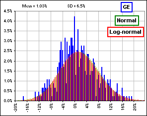
Okay, which is the better fit? Normal or Log-normal?

>zzz ZZZ
Which is the better fit?
>zzz ZZZ

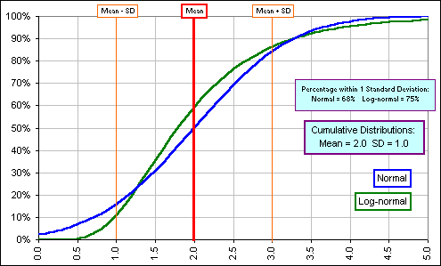
I leave you with this:

We should also note the effect of increasing the Standard Deviation on your eventual portfolio after 1, 2, 3, ... 15 years. If we look at the range of possible portfolios (within two standard deviations of the Mean Return), assuming (for example) a Log-normal distribution and SD = 15% and SD = 25% ... we get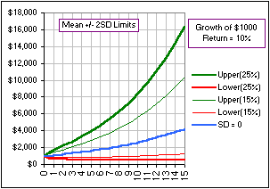

for Part II