| Magic Formulas ... and reBalancing |
I often need certain magic formulas, so I thought I'd ...
>You thought you'd stick 'em here, right?
Right.
Suppose your portfolio has annual returns of r1, r2, ... rn, over n years
... where r = 0.123 corresponds to a 12.3% return
Then the total gain is:
[1] G = (1+r1)(1+r2)...(1+rn)
... meaning that $1 grows to $G in n years
Okay, let's take the log of this guy, giving:
[2] logG = log(1+r1) + log(1+r2) +...+ log(1+rn)
... since the log of a product is the sum of the logs
| But, for small values of a number z:
[3] log(1+z) = z - (1/2)z2 + (1/3)z3 - ... In fact, if the zs are "usual" returns ... hence pretty small numbers | 
|
[4] logG = r1 + r2 + ... + rn - (1/2)(r12 + r22 + ... +rn2)
| Aah, but elogG = G and we know that:
[5] ez = 1 + z + (1/2!)z2 + (1/3!)z3 + ... Again, we ignore powers of z greater than 2 and take: ez = 1 + z + (1/2)z2 
| 
|
| [6] G = elogG | = EXP[r1 + r2 + ... + rn - (1/2)(r12 + r22 + ... +rn2)] |
| = 1 + [r1 + r2 + ... + rn - (1/2)(r12 + r22 + ... +rn2)] + (1/2)[r1 + r2 + ... + rn - (1/2)(r12 + r22 + ... +rn2)]2 ... approximately | |
| = 1 + [r1 + r2 + ... + rn - (1/2)(r12 + r22 + ... +rn2)] + (1/2)[r1 + r2 + ... + rn]2 ... ignoring higher order terms |
n-year Gains
... approximately, for small numbers rk |
Now we'll look again at [1], but this time we'll consider the annualized gain factor:
[1A] GN = (1+r1)(1+r2)...(1+rn)
... meaning that an annual gain of G gives the final value of a $1.00 portfolio, over n years
Continuing, we get (taking logs):
[2A] N logG = log(1+r1) + log(1+r2) +...+ log(1+rn)
= r1 + r2 + ... + rn
- (1/2)(r12 + r22 + ... +rn2)
= Σrk - (1/2)Σrk2
... as we did above
So
[2B] logG = (1/N) Σrk
- (1/2N)Σrk2
so that
[2C] G = exp[log(G)]
= 1 +
[(1/N) Σrk
- (1/2N)Σrk2]
+ (1/2)[ (1/N) Σrk
- (1/2N)Σrk2]2
and, since we're neglecting powers of the rk higher than "2", we get:
Annualized Returns
... approximately, for small numbers rk |
That gives:
... approximately, for small numbers rk
Note: This gives an approximation to the Compound Annual Growth Rate, namely:
CAGR = Mean - (1/2) Variance
>Approximately.
>So you're talking about a portfolio with a single stock, right?
Of course, if you just invest $x in the first asset and $y in the second (with $x+$y=$1.00), and you did NOT rebalance,
>Which is larger?
A fair question. If
>And the answer is ...taDUM!
Notice that, when x = 0% or 100%, the two CAGRs are the same. You're investing in just one asset.
>Okay, but maybe rebalancing reduces volatility.
Note:
Note that, over n years, the non-reBalanced portfolio has an annualized growth rate according to Q, where:
In contrast, a rebalanced portfolio has an annualized growth rate according to P, where:
So what does the P-chart look like:
[C] (1/P) d2P/dx2
= M2 - [VAR[Wk] + M2]
= - VAR[Wk]
Since Variance = StandardDeviation 2 is never negative, the P-curve has a negative second-derivative ... hence is concave down.
>So the maximum, with rebalancing, is somewhere between x = 0% and x = 100%, right?
We saw in an earlier investigation here , that if:
[7]
Pn = Π (1+x ak+y bk)
gives the final value of a $1.00 portfolio, With rebalancing.
then the annualized gain factor is (approximately) :
P = 1 + x a +y b
- (1/2){
x2 VAR(A) +
y2 VAR(B) +
2x y COVAR(A,B)
}
Similarly, if the annualized Gain Factors for each of assets A and B are
A and B respectively, then: and (approximately) :
[7A.a] A = 1 + a - (1/2)VAR(A)
where a and b are the average (or mean) returns and (remember!)
A and B are the annualized gain factors... for each asset.
>Aren't you changing your notation?
[8] Q = [ x An + y Bn ] 1/n
If we look at the size of the terms in, say, A = 1 + a - (1/2)VAR(A) we might get something like:
Then, as an approximation, let's use (1+z)n ≈ 1 + nz when z is small.(and n isn't too large!).
[8A.a] An ≈ 1 + na - (n/2)VAR(A)
and finally:
[8B] Q = [ x An + y Bn ] 1/n
= [ 1 + n (xA + yB) - (n/2) (x VAR(A) + y VAR(B) ] 1/n noting that x + y = 1
Now let's use (1+z)1/n ≈ 1 + (1/n)z and we'll get:
[8C] Q
= 1 + (xA + yB) - (1/2) (x VAR(A) + y VAR(B)) approximately
And now, finally, we consider the difference:
[8D] P - Q
= (1/2) (x VAR(A) + y VAR(B)) -
(1/2){
x2 VAR(A) +
y2 VAR(B) +
2x y COVAR(A,B)}
approximately
Aah, but there are terms involving x - x2 = x (1-x) = xy and y - y2 = y (1-y) = xy so we get finally:
>How many times have you said "finally"?
[9] P - Q
= (xy) (1/2){VAR(A) + VAR(B)) - 2 x y COVAR(A,B)}
approximately
>But that's the same as Bernstein's bonus ... isn't it?
>Pretty lousy, I'd say.
Look again at [7A.a] and [7A.b], namely
We'll use our new, improved approximation to get:
Then
and, using (1+z)1/n = 1 + (1/n)z, we get:
[10] Q = [ x An + y Bn ] 1/n
= 1 + (xu+yv) + (1/2)(n-1) (xu2+yv2)
Now consider P again:
If we subtract from Q from P we get, finally, the difference between the reBalanced and nonreBalanced gains:
P - Q =
(xy) (1/2){VAR(A) + VAR(B)) - 2 COVAR(A,B)}
- (1/2)(n-1) (xu2+yv2)
>I recognize that first piece. Isn't he ...?
>Uh ... what's that u and v, again?
>Everything is "approximately", right?
Okay, how big is this correction? Remember that the Bernstein "Bonus" is typically less than 1%.
>Wow! That's a huge"correction" !
>And the next correction term is ... what?
In general, I guess we should write the rebalancing bonus as:
>Enough! We're talking approximations, approximations, approximations ...
Since the Variance of a set of returns is given by:
Variance = (average of the squares) - (the square of the average)
we can replace the average of the squares, namely (1/N)Σrk2,
by Variance + (the square of the average).
That is, we can put: (1/2N)Σrk2
- (1/2)[(1/N)Σrk]2 =
(1/2)Variance
Annualized Returns
[(1+r1)(1+r2)...(1+rn)]1/N
= 1 +
(1/N) Σrk
- (1/2)Variance
= 1 + Mean - (1/2) Variance
Yes, but you can click here to play with a
spreadsheet to see how good (or bad) it is.
Wrong. I'm talking about a series of annual (or weekly or monthly) returns: r1, r2, r3, ... ...
If your portfolio is made of, say, two assets with returns
a1, a2, a3, ... ... and
b1, b2, b3, ...
and you rebalance annually to maintain a fraction x of your money in the first asset and y = 1 - x in the second asset,
then your annual portfolio returns would be:
r1 = xa1+yb1,
r2 = xa2+yb2,
r3 = xa3+yb3, ...
then, after n years, your $1.00 portfolio would be worth
x(1+a1)(1+a2)...(1+an)
+ y(1+b1)(1+b2)...(1+bn)
>Shall I ask the burning question?
reBalancing ... yes or no?
Sure. Go ahead.
Pn = (1+xa1+yb1)(1+xa2+yb2)...(1+xan+ybn)
= Π (1+x ak+y bk) ... with rebalancing
and
If Qn = x(1+a1)(1+a2)...(1+an)
+ y(1+b1)(1+b2)...(1+bn)
= xΠ (1+ak) + yΠ (1+bk) ... withOUT rebalancing
which is larger? P or Q?
It depends upon the returns, eh?
If I select 50 random returns for each of assets A and B, and pick x-fractions
(to devote to asset A), we can get
better CAGR with rebalancing, or sometimes withOUT rebalancing, or sometimes it depends upon how much is devoted to asset A.
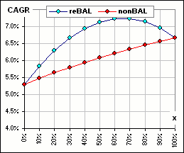
sometimes reBalancing is better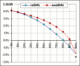
sometimes reBalancing is worser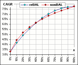
sometimes it depends upon x
These charts are available in the spreadsheet noted above 
The two sets of 50 returns are randomly chosen from Normal distributions to (sorta) mimic actual returns.
And if you regard volatility as "risk" (heaven forbid!), then it'd reduce risk, eh?
Let's try that again ... with our 50 randomly selected returns for each of assets A and B.
As before, we consider varying the fraction of asset A (that's x).
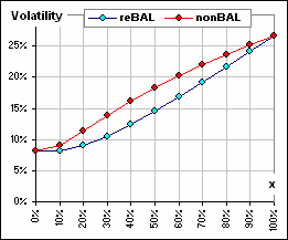
sometimes reBalancing is better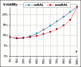
sometimes reBalancing is worser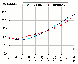
sometimes it depends upon x
These charts are available in the spreadsheet noted above 
In another tutorial
we talked about Bernstein's so-called Rebalancing Bonus.
In fact, Bernstein's "bonus" is never negative **, implying that rebalancing is good ... indeed, it's always good.
Alas, that ain't (always) the case 
**
Bernstein's "bonus" = (1/2) x y ( VAR[A] + VAR(B) - 2 COVAR(A,B) )
and, if U and V are the Standard Deviations of assets A and B, and r is their correlation coefficient, then this can be written:
Bernstein's "bonus" = (1/2) x y (U2 + V2 - 2 r U V ) ≥
(1/2) x y (U2 + V2 - 2 U V ) = (1/2) x y (U - V)2 ≥ 0
the Shape of Curves
If Qn = x(1+a1)(1+a2)...(1+an)
+ y(1+b1)(1+b2)...(1+bn)
As a function of x, that right-side is a straight line.
Pn = (1+xa1+yb1)(1+xa2+yb2)...(1+xan+ybn)
and that right-side ain't hardly a straight line!
However, the P-chart starts and ends at the same point as the Q-chart
... when x = 0% and x = 100%
We'll do a wee bit o' calculus here:
>Wake me when you're finished ...
[A] (1/P) dP/dx = (1/n) ΣWk ... from 3
[B] (1/P) d2P/dx2=
[(1/n)ΣWk]2
- (1/n) ΣWk2 ... from 5
Let M = (1/n)ΣWk be the mean of the W's.
Then we can rewite things like so:
Then we can rewrite [B] above, like so:
(1/n) ΣWk2 =
(1/n) Σ(Wk - M + M)2
= (1/n) Σ(Wk - M)2 + (1/n) 2M Σ(Wk - M) + (1/n) ΣM2
= (1/n) Σ(Wk - M)2 + (1/n) 2M 0 + (1/n) (n M2)
... noting that Σ(Wk - M) = 0 since M is the mean of the Ws.
= VAR[Wk] + M2
...where VAR is the Variance (or StandardDeviation2) of the Wk
That means that, with rebalancing, the P-curve begins and ends at the points where the Q-curves begins and ends,
but is concave down, so ...
Sometimes ...

the "REAL" Bonus
An = Π (1+ak)
and
Bn = Π (1+bk)
[7A.b] B = 1 + b - (1/2)VAR(B)
Uh ... yeah, to keep you awake.
Anyway, it's not reasonable to compare P to x A + y B since the latter doesn't represent the gain factor of the nonreBalanced portfolio.
Indeed, the nonreBalanced portfolio has an n-year gain of x An + y Bn, hence an annualized gain factor of:
1 + 0.08 - (1/2)(0.02) = 1 + 0.08 - 0.01 = 1 + 0.07
so it's very near the value 1.0
That'd give:
[8A.b] Bn ≈ 1 + nb - (n/2)VAR(B)
Pay attention!
We now have the "real" rebalancing bonus:
Uh ... yes, so it is.
I guess that (1+z)n = 1 + nz isn't such a good approximation.
Let's check:
z = 0.1, n = 30 (1+z)n = 17.4 1 + nz = 4
z = 0.1, n = 10 (1+z)n = 2.6 1 + nz = 2
z = 0.1, n = 5 (1+z)n = 1.6 1 + nz = 1.5
Yeah, that approximation is like using simple interest rather than compounding the returns.
I guess the moral is that you may get Bernstein's rebalancing bonus for the short term, but ...
>And the long term?
Okay, let's investigate. First, we note that:
z = 0.1, n = 30 (1+z)1/n = 1.0032 1 + (1/n)z = 1.0033
z = 0.1, n = 10 (1+z)1/n = 1.0096 1 + (1/n)z = 1.010
z = 0.1, n = 5 (1+z)1/n = 1.019 1 + (1/n)z = 1.020
>So using (1+z)1/n = 1 + (1/n)z is good, eh?
Yeah, so now we'll use an improved approximation for (1+z)n, namely (1+z)n ≈ 1 + n z + (1/2)n(n-1)z2
[7A.a] A = 1 + u ≈ 1 + a - (1/2)VAR(A) where u is the annualized return
[7A.a] B = 1 + v ≈ 1 + b - (1/2)VAR(B) where v is the annualized return
[8A.a] An ≈ 1 + n u + (1/2)n(n-1)u2
[8A.b] Bn ≈ 1 + n v + (1/2)n(n-1)v2
xAn + yBn = 1 + n (xu+yv)
+ (1/2)n(n-1) (xu2+yv2)
putting x + y = 1
P
= 1 + x a +y b
- (1/2){
x2VAR(A) +
y2VAR(B) +
2xy COVAR(A,B)
}
= 1 + x [ u + (1/2) VAR(A) ]
+ y [ v + (1/2) VAR(B) ]
- (1/2){
x2VAR(A) +
y2VAR(B) +
2xy COVAR(A,B)}
putting a = u + (1/2)VAR(A) and b = v + (1/2) VAR(B)
= 1 + x u + y v + (1/2) x y { VAR(A) + VAR(B) - 2 COVAR(A,B) }
putting x - x2 = y - y2 = xy
Bernstein's Rebalancing Bonus? Yes. Interesting, eh?
But now we have an extra "correction", namely (1/2)(n -1) (xu2+yv2)
They're:
u = a - (1/2)VAR(A)
v = b - (1/2)VAR(B)
which are the annualized returns for assets A and B ... approximately
Yes.
If the annualized returns u and v are, say about 8% (or 0.08) then the correction is about
(1/2)(n -1) (x 0.082+y 0.082)
and, for a 50-50 allocation (so x = y = 0.5) and n = 10 years, we'd get something like 3%.
Ain't it though ... and maybe the next correction would be even larger 
I think it's (1/3!) (n-1) (n-2) (xu3+yv3) so, for n = 10 and x = y = 0.5, this is about 1%.
Note that the terms get smaller when (1/m!) nm-1 um and (1/m!) nm-1 vm are small.
Rebalancing Bonus =
(xy) (1/2){VAR(A) + VAR(B)) - 2 COVAR(A,B)}
- (1/2!)(n-1) (xu2+yv2)
- (1/3!) (n-1) (n-2) (xu3+yv3) + ...
For example, for n = 10 and u = 0.08, then
(1/m!) 10m-1 0.08m = 0.0032 when m = 2
and (1/m!) 10m-1 0.08m = 0.0085 when m = 3
and (1/m!) 10m-1 0.08m = 0.0017 when m = 4
and ...
Uh ... yes, but I think we can conclude that the "bonus" is reduced for assets that are highly correlated
(so COVAR(A,B) is large) and whose annualized returns are large
(so u and v are large).

