the Kalman Filter

Every so often I get email asking about the Kalman filter and ...

>And you know nothing about it, right?
Uh ... not exactly, but I reckon it's about time to write about it since it seems to be popular these days in financial stuff.

Rudolf Emil Kalman, born in 1930 in Hungary, was trained as an Electrical Engineer.
He is most famous for the Kalman filter, a scheme for extracting a signal from a series of noisy (or incomplete or corrupted or chaotic) measurements.
His original 1960 paper was, apparently, received with scepticism. It is now a popular prescription for extracting a signal from a noisy environment.

He is a member of the National Academy of Sciences (USA), the National Academy of Engineering (USA), and the American Academy of Arts and Sciences (USA).
He is also a foreign member of the Hungarian, French, and Russian Academies of Science and has numerous honorary doctorates.

>Are we talking electrical engineering?
Not at all.

• Suppose you wanted to measure the level of water in a large tank. The surface sloshes about and there's water flowing into the tank.
• Suppose you want to know your position at sea and you take measurements of star positions. Your readings have noise.
• Suppose you wanted to know the position of a moving object captured by two radars. The object is moving. There's noise in the radar images.
  You use the radar info to estimate the possible range of positions at some time t. Theres a probability distribution associated with this position.
  Do you accept the average? The median? The position of maximum probability?
• Suppose ...

>I'd accept the Kalman position. Am I right?

Patience. Note that there's a range of possible answers to your question: "What's the value of x?" The probability that the true value of x is L will depend upon the measurement(s) you've taken. That makes it a "conditional probability". If you've measured the level of water as z1 = 123 metres, then it's unlikely that the "true" level is x = 500 metres. There's a distribution of possible x-values which, we'd expect, would vary about z1 = 123 metres. Indeed, with a single measurement we'd expect a range of values like the blue curve in Figure 1. That's probably the best you can do with a single measurement. It's your best estimate. It's centred on z1 = 123 metres. (For our example, we've picked a Standard Deviation of 15 and a Normal distribution.) Aah, but suppose you take a second measurement: z2 = 142. Suppose, too, that you know that this second measurement is more accurate. There's a distribution about z2 = 142 perhaps like the green curve in Figure 1. It's more congested near 142, more compact, less spread out ... because 142 is presumably a better estimate. 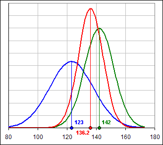(We've picked Standard Deviation = 10 and a Normal distribution.) Here comes the big question: What does the x-probability distribution look like if two independent measurements gave the blue and green distributions in Figure 1? That is, what's the conditional probability, given the probability distributions for z1 and z2?

Figure 1

In fact, we'd get the red distribution in Figure 1.
It's less spread out then either of the two other distributions.
Indeed, if the two other distributions have Mean values of M₁ = z₁ and M₂ = z₂ and Variances of V₁ and V₂, then the red distribution will have:

[1]   Mean = (V2 z1 + V1 z2) / (V1+V2) = ( z1/V1 + z2/V2) / (1/V1+1/V2)     and     1/Variance = 1/V1 + 1/V2

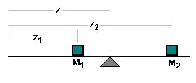
>Mamma mia! Is that really necessary? That looks bad and ... The resultant Mean for the red distribution is just a linear combination of z1 and z2. Look at it this way: You have two objects, with masses M1 and M1. They're on a seesaw and you want to balance the seesaw by placing a fulcrum at the right spot so as to balance the two weights. The balance point must be placed so that the total mass, concentrated at its location, has the same moment about one end point.

Figure 2

That'd require:
M₁ Z₁ + M₂ Z₂ = (M₁+M₁) Z hence: Z = (M₁ Z₁ + M₂ Z₂) / (M₁+M₁)
See the similarity?

>No! Besides, you're calling the masses M₁ and M₂ and that's what you called the Means, earlier.
Uh ... sorry about that, but it's necessary to keep you awake.

Anyway, just replace the masses like so: M₁ = 1/V₁ and M₂ = 1/V₂ and the two formulas are the same.
The reciprocals of the Variance play the role of masses. That makes sense, right?
After all, the red distribution is supposed to combine the blue and green distributions and you'd expect the resultant Mean would be closer to the Mean with the narrower distribution, since that's presumably the more accurate measurement. Then, too, the "total mass" is the sum of the two individual masses, making 1/Variance = 1/V₁ + 1/V₂.

Remember: Variance = (Standard Deviation)².

In our Figure 1 example, we've chosen M₁ = 123 and V₁ = 15² = 225 and M₂ = 142 and V₁ = 10² = 100.
That'd give (for the red distribution):
Mean = (100*123 + 225*142)/(225+100) = 31%(123) + 69%(142) = 136.2   and   1/Variance = 1/225+1/100 = 0.01444 so the Standard Deviation = 1/SQRT(0.01444) = 8.32.
In particular, notice that the red distribution is narrower inplying more confidence in the 136.2 estimate and ...

>Wait! You make a single measurement like 123 and you automatically get a distribution and you automatically know that your second measurement is more accurate and ...
Patience. We'll get to all that stuff soon enough.
In the meantime, let's assume that we DO have an estimate for the Standard Deviations of our two measurments
and that we DO adopt a Normal distribution with Means z₁ and z₂ and Variance estimates of V₁ and V₂.
Our analysis would then proceed as we've done above.

Of course, these assumptions should be reasonable, right? But look at the implications:

1. If each measurement were equally accurate, the two variances would be equal and the conditional Mean would the the average of the two Means: (z₁+z₂)/2.
2. If one measurement were more accurate, the conditional Mean would be closer to that measurement.
3. The conditional Variance is always less-than-or-equal-to than the individual variances. That implies that every additional measurement increases the accuracy of our result.

Kalman Dynamics

Let's rewrite the magic formulas [1] like this:

[a]     Mean = z₁ + [V₁/(V₁+V₂)] ( z₂ - z₁)     and     Variance = V₁ - [V₁/(V₁+V₂)] V₁

In other words, we can write:

[b]     Mean = z₁ + K₂ ( z₂ - z₁)     and     Variance = V₁ - K₂ V₁     where K₂ = [V₁/(V₁+V₂)].

We now imagine taking our first measurement at time t₁ and our second measurement at time t₂.
Further, let's call X₁, X₂, etc. the increasingly accurate estimates of the Mean as we take more measurements.
We'll let U₁, U₂, etc. be the successive estimates of the Variance.
After the first measurement of z₁, our "best" estimates are X₁ = z₁ and U₁ = V₁.
After the second measurement at time t₂ our best estimate is obtained from [b], above:

[c]     X₂= z₁ + K₂ ( z₂ - X₁)     and     U₂ = U₁ - K₂ U₁

Do you see where we're heading?

>No! It's mumbo-humbo. You're just ...
We're marching ahead in time and, at each step, trying to predict the value (and associated distribution) of some variable.

>The value of what variable?
Maybe it's the alpha or beta of a stock or maybe the inherent Volatility or maybe ...

>Please proceed.
Okay, we'll assume that the "true" values of our variable are x(t₁), x(t₂), x(t₃) etc.
Further, we assume they evolve in time according to the following prescription:

[d]     x(t_n+1) = F(t_n) x(t_n) + w(t_n)     where w is random noise.
That is, each new value depends upon the previous value ... but there's some random variation introduced by the variable w.

Our observed (that is, "measured") values are z(t₁), z(t₂), z(t₃) etc. and they evolve in time according to the following prescription:

[e]     z(t_n+1) = H(t_n) x(t_n) + v(t_n)     where v is random noise (or "error").

We'd like to get at the "true" x-values by looking carefuly at our sucessive z-observations and ...

>With all that noise?
We have to make some assumptions about the noise.
In fact, we'll assume the noise is sometimes positive, sometimes negative but the average noise is zero.
In fact, we'll assume the noise is selected at random from a Normal distribution with Mean = 0 (and some as-yet-unspecified Variance).
In fact, we'll also assume the two random noise terms, w(t_n) and v(t_n), are independent.
In fact, we'll assume that after having made an observation like z(t_n) we estimate the "true" value of x(t_n+1) in terms of a conditional probability, given that we've just added a new z-observation.
In fact ...

>Can you just continue?
Okay. Notice that we're trying to generate a "best estimate" of the true x-values by using the z-observations and, at each step, we (hopefully) improve our estimate recursively.

>Recursively?
Yes. We don't go back and look at all the observed z-values, but just update at each time step.
That's like calculating an average by using: A_n = (1/n) (a₁ + a₂ +...+ a_n).
We use, instead: A_n = (1/n) [ (n-1)A_n-1 + a_n ]. That way we can update A without looking at all previous a-values.
Then, too, if we make assumptions about the noise in our Kalman filter, w(t_n) and v(t_n), we'll have their covariances ... in advance.

Finally, we want our z-estimates to be such that their average over time approaches the "true" x-values.
In fact, we want a procedure such that our z-estimates give, on average, the smallest estimation error.

>You're dreaming ...
Actually, Kalman does just that: of all such algorithms it gives the "best" estimate in the sense that the mean-square error is minimized.