I've never been enthusiastic about the common assumptions that stock returns are distributed normally or lognormally or ... whatever.
(See this or this.)

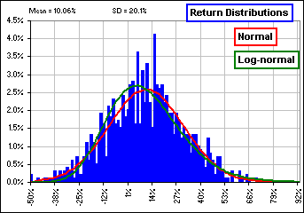
For example, the normal and lognormal distributions look like Figure 1a. The normal density distribution is described by: [1]         and the lognormal by: [2]         Figure 1b gives a fit to S&P 500 returns. >Looks pretty good to me! Just wait. Note that, in the lognormal distribution, log(x/G) = log(x) - log(G) = log(x) - m, hence involves a variable of the form: u = (something - m)/S. >So does that normal guy, right? Yes. Pay attention. The cumulative distribution (being the area beneath the density function f(x)), is always an increasing curve which varies from 0 to 1 (or 0% to 100%). So here's an interesting idea: Let K(u) be an increasing function of u. Define z = A + B K(u). Pick A and B so z varies between 0 and 1. Set u = (x - m)/S and you've got yourself a cumulative probability.

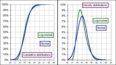Figure 1a Figure 1b

>Example?
Here are a few increasing functions for z :

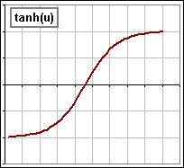hyperbolic tangent	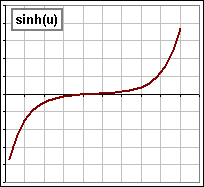hyperbolic sine	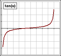tangent
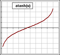inverse hyperbolic tangent	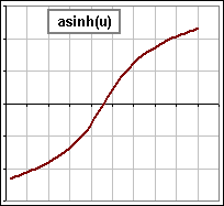inverse hyperbolic sine	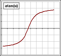inverse tangent
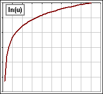logarithm	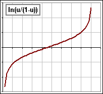log-ratio	inverse hyperbolic sine

... and a few curves of the form  
>That inverse hyperbolic sine ... you've got it twice.
So I have. It's a good one. Anyway, here are the curves:

using the hyperpolic tangent

using the inverse hyperpolic sine

using the inverse tangent

>What's this Johnson stuff?
N.L. Johnson, in 1949, generated a bunch of probability distributions with several parameters (like our A, B, m and s) and ...

>And you want to generate a few yourself, eh?
Well, I'd like to describe the Johnson curves, but first we note the following:

• If z is a normally distributed random variable, then it's described by the function: e^-z2/2
• If z = (x-m)/s, this describes is a normal distribution for the random variable x, with mean m and standard deviation s.
• If z = (log(x) - m)/s, this would give a lognormal distribution for x.
• We note that (x-m)/s and (log(x) - m)/s are both increasing functuions of x.
• If we introduce any increasing function we might expect to get some sort of distribution.

Johnson Distributions

We fiddle with a normal distribution to generate various other distributions
>Fiddle?
Yes, we stretch and slide and generally distort a normal distribution, like so:

• First, consider a normal distribution, N, described by:
       
   
• Then we introduce a magic function of our choosing (which we'll call J):
        z = A + B J(u) where u = (x-m)/s.
   
• If we plot N(z) versus z, we'd get the familiar normal distribution,
  but if we plot N versus u we'd get something else ... depending upon our choice of J
   
• Now consider N versus x (where u is just the x-variable, moved left or right and scaled)
   

The Johnson-modified normal curves then look like this:

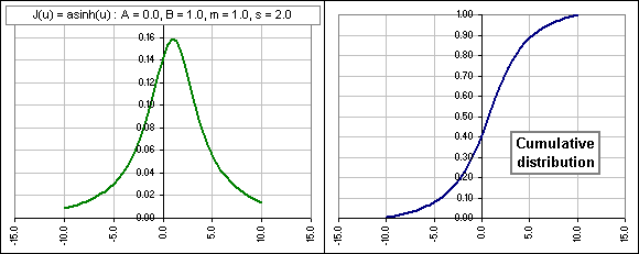
J(u) = inverse hyperpolic sine

J(u) = log(u/(1-u)) ... which requires m < x < m + s

J(u) = log(u) ... which requires x > m

J(u) = u ... that's your standard, garden variety normal distribution

Note that, if
      z = A + B J((x-m)/s)
then, solving for x, we get:
      x = m + s J^-1((z-A)/Bs)
where J^-1 is the inverse of the J-function.

For example, if J(u) = sinh(u), then we'd get:
      z = A + B sinh((x-m)/s) and x = m + s sinh^-1((z-A)/B)

The problem, of course, if to identify the parameters A, B, m and s so that whatever curve we choose, it matches historical data as closely as possible. That usually means matching the first four moments.

>Huh?
We note that, if z is a random variable (running, say, from -infinity to infinity) with density distribution f(z),
then the first four moments are given by:
        and     and     and  

>Is that hard?
We'll see, but in the meantime, here's a fit to 30 years S&P 500 monthly returns:

To play with these curves, you can fiddle with a spreadsheet which looks like this:

You can type in some stock symbol (a la Yahoo)
... then vary A, B, m and s to see how well you can fit a Johnson (or other) distribution.
(There are up and down buttons to control these values ... to make life easier.)  

>Or other?
Yes. You define some J(u), click the button and your J(u) is inserted into the spreadsheet.

You also get the cumulative distribution associated with your chosen J(u), so you can specify some return and get the probability that the stock return will be less than that.
In the picture above, a 1.5% return is selected. The probability is 98%, using the lousy distribution shown .
It's interesting to see how this changes with your choices of the four parameters !!

After you play with the UP and DOWN buttons, you can click on a couple of buttons and the spreadsheet will attempt to find the "best" parameters.
>Complicated!
Well ... there's an Explain sheet.

To download the spreadsheet, click on the picture, or, if that don't work, RIGHT-click and Save the target link.
Note: the spreadsheet may be different than shown above  

click for Part II