| Central Limit Theorem: Introduction |
|
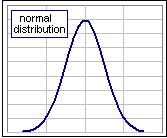
There's this theorem that explains why the Normal (or Gaussian) distribution crops up so often. >Don't tell me! It's the central limit thing, right?
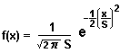
Consider some (unknown!) probability density function f(x). (We'll refer to it as pdf).
|   |
|
Then we note the following, in Table 1: ... where the integration is over all possible values of the (random) variable x, say: -∞ to +∞. >Okay, all those guys have names. So?
|
|
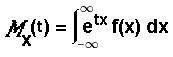
| Okay, now consider the following integral: |
|

Expanding etx in a Taylor series, we get:
| [2a] Mx(t) = ∫ (1 + tx + t2x2/2 + ...) f(x) dx
= 1 + Mt + S2t2/2 + ...
= 1 + S2t2/2 + ...
using Table 1, noting that M = 0 for the case we're considering. |
For that reason Mx(t) is called the Moment Generating Function.
>Moments? Why are they called moments?
Uh ... let's recall something about moments of a force about a point.
|
Imagine a bunch of weights on a board, like so: The "moment" of each about the left end of the board is: (weight)*(distance to the left end). The total moment of all the weights is the sum of these moments. Suppose the weights (at distances x1, x2, etc.) were f1, f2 ... | 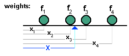 Moments of forces about a point |
The total moment is then: f1 x1 + f2 x2 + ... and we want to know where to put a fulcrum in order to balance all them weights on the board.
It'd be a place where the total weight would have the same total moment. That is, we'd want:
[A] (f1 + f2 + ... )*X = f1 x1 + f2 x2 + ...
See that right side? It looks just like #3 in Table 1, eh?
|
>Except that you're summing instead of integrating, right?
Yes. However, if the weights were not discrete but uniformly distributed along our board, we'd integrate. | 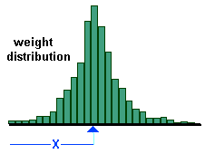 Moments of forces about a point |
If all the weights were equal to 1 (so the sum equals n), then [A] says:
[B] n X = x1 + x2 + ... +xn
which says we should place our fulcrum at: X = ( x1 + x2 + ... +xn) / n.
>That's the average distance. I knew that!
Good for you.
In [A] we've summed fj xj, but we could also sum fj xj2
(the second moment) or maybe fj xj3 or maybe ...
>Yeah, I get it.
That second moment (for the weights on our board) has a name: Moment of Inertia and Engineers use it all the time to determine the strength of beams.
For example, the I-beam is designed so that ...
>Could you get back to ... uh, what were we talking about?
Sorry. Let's continue.
The magic formulas [1] and [2a] define the Moment Generating Function. Note the following:
|
[i] If we know the distribution function f we can calculate Mx(t).
[ii] Further, if we know Mx(t) we can calculate the pdf, f. |
Now let's enumerate some interesting characteristics of our Moment Generating Function:
|
>Wait! What's that about? When you add random variables you multiply the generating functions together?
This relationship, where sums get replaced by products or products get replaced by sums ... it's familiar.
Remember that the logarithm of a product is the sum of logarithms.
Check out Stat Stuff 4.
If you multiply uncorrelated, independent random variables, the Mean of the product is the product of the Means.
Hence, the Mean (or Expected) value of the product ex tey t is the product of the two Expected values:
Mx(t) and My(t).
| Central Limit Theorem: Proof |
Okay, now consider the Variance of an Average (or Mean) of n independent / uncorrelated random variables selected from the same distribution.
We assume that distribution has Variance S2 (where S is the Standard Deviation).
>Huh?
We're picking n random values and averaging them. Then we pick another n and average them. Then another and another.
We look carefully at all the averages we've calculated and ask: "What's the distribution of all these averages?"
>But you need to know the distribution of the random values ... don't you?
Patience. The result is really quite remarkable. 
We first inspect Stat Stuff 8.
If they're independent, the Variance of a sum is the sum of the Variances. Hence:
[C1] Var[ (x1 + x2 + ... + xn) / n ] = Var[ x1 / n ] + Var[ x2 / n ] + ... + Var[ xn / n ] = (1/n2) Var[ xk] ... using Stat Stuff 2
Continuing:
[C2]
Var[ (x1 + x2 + ... + xn) / n ] = (1/n2) (n S2) = S2 / n
... since the variance for all selected random variables is the same, namely S2.
If the Variance is S2 / n, then the Standard Deviation is S / √n.
We're interested in the pdf distribution of these averages. Let's call the collection of averages Yn.
A "typical" value would look like: Yn = (x1 + x2 + ... + xn) / n.
Now, if we knew the Moment Generating Function for these averages we would know their distribution.
To this end we consider related "normalized" variables:
[D1] Zn = Yn / (S/√n) ... where a typical value looks like: Zn = { (x1 + x2 + ... + xn) / n } / (S/√n) = (x1 + x2 + ... + xn) / (S√n).
Note that the Zn are sums of n terms each looking like: xj / (S√n).
Then their Moment Generating Function is a product of n Moment Generating Functions, each looking like:
[D2]  ... using Table 2.1 stuff.
>zzzZZZ
Don't you see? It's just a matter of changing the scale for t. We replace t by t / (S√n).
Remember that we want the product of all n of these generating functions.
Since all the xs are chosen from the same distribution, the generating functions will all be the same.
Hence and therefore (I love that phrase!):
[D3] MZn = { Mx(t /S√n }n
Do you remember [2a]?
>And that red curve?
>zzzZZZ
The pdf for these numbers looks something like this:
>zzzZZZ
Well, now it comes in handy. We're going to change to t / (S√n) and consider
That means that t / (S√n) is small. That means that we can rewrite [2a] like so:
Now here's a neat thing to know:
[2b]
MZn
= {1 + t2/2n + ...}n
where we've replaced t by t / (S√n) and set the Mean M = 0.
The limit of (1 + k/n)n as n → infinity is ek.
Now stare carefully at [2b] and assume all them neglected terms are really, really small compared to the term t2/2n
... then wave our magic wand and get, for large samples:
[3]
MZn
![]() et2/2 as n
et2/2 as n ![]() infinity.
infinity.
>zzz ... huh? Is that it?
Yes. We have the Moment Generating Function of the distribution of averages (for large samples), taken from the same (almost) arbitrary distribution.
>And that gives the Central Limit Theorem?
Yes, because we know the generating function (for large n) hence we know the probability density distribution (for large n) ... and that's the Normal Distribution.
 I forgot to mention that the Moment Generating Function for the Normal distribution is nobody else but et2/2.
Remember, Normal distribution pdfs contain a factor like: e-x2/2 ... and I leave the integration of ext e-x2/2
= et2/2 e-(x-t)2/2 up to you.

Central Limit Theorem: Examples
I should also mention an example or two:
>So you regard 5000 as a large value for n?
Let's pick 50 random numbers uniformly distributed in the interval (0,1) ... using RAND(), in Excel.
The pdf for these uniformly distributed numbers looks like this: 
Now we randomly select 50 from this distribution and calculate their average.
Then we repeat this 5000 times and plot the frequency with which averages occur.
Then we'd get something like this ![]()
I'll give you one guess. 

No, I regard n = 50 as a large value for n. Those 5000 average calculations are just to get the distribution of the n-value averages.
Have you been paying attention? For large n, the distribution of these averages approach a Normal distribution.
The more averages you compute, the better the picture of the distribution:


Now we consider random numbers that are either 0 or 1, with equal probability
... using IF(RAND()<0.5, 1, 0).

Again, we select 50 at random and average them.
We repeat this 5000 times and plot the distribution of the averages ... and get this: ![]()

Now we consider random variables that are generated like so:
We can use the Excel function IF(RAND()<RAND(), RAND(), NORMDIST(RAND(), RAND(), RAND(), 0)).
It'll give the random variables described above.
The pdf for these variables looks something like ... uh ... I have no idea. 
When I do this, I get Figure 1. Does it look normal?
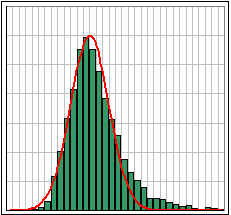
Figure 1