Bollinger Bands: Introduction

Years ago, when I first ran across Bollinger Bands, I thought they were pretty neat ... stock prices bouncing between two curves, the Upper and Lower boundaries of the "band" and ...
>Remind me. Bollinger bands?
We look at the last n stock prices P₁, P₂, ... P_n (where we include P_n, today's price, and where P₀ is the price n days ago) and we calculate their average, P_av, and their Standard Deviation, SD:

Pav = (1/n)(P1+ P2+ ... +Pn) = (1/n)ΣPk       SD2 = (1/n) [ (P1-Pav)2+ (P2-Pav)2+ ... + (Pn-Pav)2) ] = (1/n)ΣPk2 - Pav2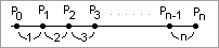

(See SD stuff.)

Then, each day, we plot the two points:

[a]       U = Pav + k SD [b]       L = Pav - k SD These points trace out two curves and we see the current stock price bounce between the two curves, U and L, as in Figure 1. >So what are n and k? You can pick anything., but we'll choose n = 20 days and k = 2 standard deviations. >So you buy at L and sell at U? I didn't say that!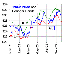

Figure 1

>So what are you saying?
I just want to look at Bollinger Bands, again, because although one often calculates the SD (or Volatility) of stock returns, it's strange to see the SD of stock prices and ...
>As in Bolli bands?
Yes, as in Bollinger Bands. We did, at one time, try to find a relationship between the statistical properties of returns and of prices, here. What we want to do now is investigate WHY one would expect stock prices to oscillate between U and L.

When we consider the SD of daily returns, we often assume they have a Normal distribution ... in which case it's unlikely that returns will lie too far from the Mean return. In fact, we would expect most returns to lie within 2 Standard Deviations of the Mean return. In fact, if they were Normally distributed, the probability that the returns lie within two SDs of the Mean is X%. However, if we consider prices, do we also expect them to lie (mostly) within 2 Standard Deviations of the Mean price P_av?
>That'd be like choosing k = 2, eh?
Exactly! When today's price is larger than U or smaller than L, then it's outside that 2S band centred on P_av ... so we might expect tomorrow's price to return to the band. That says something about tomorrow's price, eh?
>And the last n = 20 prices are Normally distributed?
Ay, there's the rub! Are they?
>Huh? You're asking me?
That was a rhetorical question ... but it indicates what we want to investigate in this tutorial.

the Distribution of Stock Prices

Suppose that, over the last n days, the daily Gain Factors are g₁, g₂, g₃, ... g_n.
>Gain Factors?
Yes, if a stock price goes from $P to $Pg in a day, then g is the Gain Factor for that day.
For example, g = 1.056 corresponds to a 5.6% daily return.

Then n successive daily stock prices (after the starting price of $P₀) are P₀g₁, P₀g₁g₂, P₀g₁g₂g₃, ... P₀g₁g₂g₃...g_n
... the last being today's stock price.

So here's the question:

If the g's are selected from a Lognormal distribution, what's the distribution of the numbers g1g2g3...gn ??

>Lognormal? I thought you wanted Normal?
Well, it's common practice to consider daily gains (or, in our case, Gain Factors) to be Lognormally distributed.
Besides, it makes the math easier.  

Note that, if the g's are Lognormally distributed, then y = log(g) is Normally distributed. We'll let F(x) be the cumulative Normal distribution function for the y's. That means that the probability that a randomly chosen y is less than some x is F(x) (as in Figure 2). That's for a single random Gain Factor. What we now want is to consider the product of n such (random) Gain Factors: For any x and n random g's, what is the probability that g1g2g3...gn < x ? That requires that log(g1g2g3...gn) < log(x). That requires that log(g1)+log(g2)+...+log(gn) < log(x).

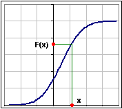Figure 2

But, as we've said, if the g's are Lognormally distributed, then y = log(g) is Normally distributed.
Hence, we set log(g_k) = y_k and ask:
What is the probability that, for a randomly selected set of y's:
     y₁ + y₂ + ... + y_n < log(x)   where the y's are Normally distributed ?
Let's label the statistical properties of the y's:
[1a]       Mean[y] = Mean[log(g)] = M
[1b]       Variance[y] = Variance[log(g)] = Var = S²   the square of the standard deviation

Now, if the g's are independent random variables (meaning zero correlation between the g's), then the y's will also be independent in which case the sum Σy_k will be Normally distributed with Mean and Variance (= SD²) given by:
[2a]       Mean[Σy_k] = ΣMean[y_k] = n M   the Mean of a Sum = the Sum of the Means
[2b]       Variance[Σy_k] = ΣVariance[y_k] = n Var = n S²   the Variance of a Sum = the Sum of the Variances (for zero correlation)
>The Mean of a sum equals the sum of the Means?
Yes, and that goes for Variance, too ... if there's zero correlation between the y's.

Okay, we now see that, since log(g₁g₂g₃...g_n) = Σy_k is Normally distributed, then g₁g₂g₃...g_n is Lognormally distributed.
>Isn't g₁g₂g₃...g_n today's stock price?
Well, yes ... after multiplying by the starting stock price n days ago, namely P₀.

Okay, our assumptions and results are, so far:

Results The price n days ago is given as P0. The daily Gain Factors, g, have a Lognormal distribution with Mean[g] = M and Variance[g] = Var = S2.       These are calculated from historical returns. The logarithms of the g's have Mean[log(g)] = M and Variance[log(g)] = Var = S2   that's [1]. The relation between the Mean and Variance of g and those of its logarithm, y, is given by:       Mean[log(g)] = M = log(M) - (1/2)S2       Variance[log(g)] = Var = S2 = log(1 + S2 / M2)       (This assumes a Lognormal g-distribution: see this.) The n-day Gain Factor is Lognormally distributed so the distribution of today's prices, Pn is Lognormal with (assuming zero correlation between daily gains):       Mean[Pn / P0] = Mean[g1g2g3...gn] = Mean[g1]Mean[g2]...Mean[gn] = Mn   the Mean of a Product = the Product of the Means       Variance[Pn / P0] = Variance[g1g2g3...gn] = (M2+S2)n - M2n     See this

>The "distribution" of today's price? But we KNOW today's price so why ...?
It gives the distribution of prices (for today), assuming a given price n days ago (that's P₀) and n random Gain Factors over the past n days. What we want is to determine the probability that today's price is within, say, 2 Standard Deviations of the average price over the last n days (that's P_av). In other words, we want the probability that today's price is inside the Bollinger Bands ... then we'll look up today's price and see where it's at.

Probability that Today's Price lies within some interval centred on the n-day Mean: Pav

Notice that, if P₀ = $1.00, then the Gain Factors g₁, g₁g₂, g₁g₂g₃ etc., are just the subsequent stock prices.
We'll assume that's the case.
>Huh? What's the case?
That P₀ = $1.00 so the products g₁g₂...g_k are the stock prices. We'll stick P₀ in our formulas ... later.

Okay, we have that today's price P_n = g₁g₂...g_n is Lognormally distributed with a known Mean and Variance as given is Results #5.

Now we ask:

If the random variable G has a Lognormal distribution with given Mean and Variance, what is the probability that G < x ... for a given number x ??

>You're asking me?
That was a rhetorical question. Now pay attention. We've been here before.

• If G < x then log(G) < log(x)
• Since G is Lognormal then log(G) is Normal
• The distribution of log(G) is then described by N[u,Mean,SD]
      the Normal cumulative distribution function
      and Mean and Standard Deviation are the Mean and Standard Deviation of log(G) ... not of G itself!
• The probability that log(G) < log(x) is then N[log(x),Mean,SD]
• But log(G) < log(x) is the same condition as G < x so the probability is the same:   N[log(x),Mean,SD]

>So the chances of being in that Bollinger band is ... what?
If A is the probability of being less than U and B is the probability of being less than L, then ...
>It's B - A, eh?
Actually, it's A - B as in: N[log(U), nM, SQRT(n)S)] - N[log(L), nM, SQRT(n)S)]

Note:

• Remember that we're talking about the probability that the n-day Gain Factor lies between two numbers.
• Don't confuse Gain Factors with daily returns.
• In fact, a Gain Factor is 1 + (daily return).
• The Mean of the Gain Factors, that's M, is "1" greater than the mean of the daily returns.
• If the Mean of the daily returns is 0.0123 (that's 1.23%), then M = 1.0123.

>When are you going to insert some other starting price ... P₀?
Other than $1.00? Right now.
The numbers U and L given in [a] and [b] assume an arbitrary P₀ value.
To generate the appropriate numbers for the case P₀ = $1.00, we'd divide each of U and L by P₀.
Assume we've divided U and L by P₀. We'll call these U' = U/P₀ and L' = L/P₀, okay?
Now we're talking about the case where P₀ = $1.00 (as we did above).
As we've seen above, the probability that G = P_n/P₀ < U' is N[log(U'), nM, SQRT(n)S)]
But U' = U/P₀ so P_n/P₀ < U' is the same condition as P_n < U.
If we then want the probability that P lies within the Bollinger Band for arbitrary starting Price, then ...
>Why don't you just give the result, okay?
Here it is:

Magic Formula Given the stock price n days ago, P0, and assuming n random daily Gain Factors which are Lognormally distributed with Mean = M and Standard Deviation = S then the probability that today's price, P, will lie within the Bollinger band: is given by:       Prob[L < P < U] = N[log(U/P0), nM, SQRT(n)S)] - N[log(L/P0), nM, SQRT(n)S)]       where N[x, Mean, SD] is the Normal cumulative distribution function, and       M = log(M) - (1/2)S2       S2 = Var = log(1 + S2 / M2)

Remember: the probability (in the Magic Formula ) is really the probability that the Gain Factor (over n days) lies between L/P₀ and U/P₀.
That's like: Prob[L/P₀ < P/P₀ < U/P₀].
If, for example, both L and U are less than the starting Price of P₀ (n days ago), then you're asking for the probability that, after n random gains, the price today has dropped to some range of lower values. Similarly, if both L and U are greater than the starting Price ...
>Do you have an example?
Okay, we'll consider the stock prices of GE over the past n = 20 days.

• Twenty days ago the price was P₀ = $15.95
• The Mean and Standard Deviation of GE daily Gain Factors are   (over the past few years):
        M = 1.023   meaning an average daily gain of 2.3%
        S = 0.014   meaning the SD of daily gains is 1.4%
• That makes:
        M = log(M) - (1/2)S² = log(1.023) - (1/2)( )² =
        S² = log(1 + S² / M²) = log(1+0.014² /1.023²) =
• The Upper and Lower Bollinger Bands (assuming k = 2 Standard Deviations) are, as per [a] and [b]:
        U = P_av + 2SD(prices) = $17.49
        L = P_av - 2SD(prices) = $13.65
• We calculate:
        log(U/P₀) = log(17.49/15.95) = ???   and   log(L/P₀) = log(13.65/15.95) = ???
        nM = 20*M = MM   and   SQRT(n)S = SQRT(20)*S = SS
• The probability that today's price lies between L = $13.65 and U = $17.49 is then
        N[log(U/P₀), nM, SQRT(n)S)] - N[log(L/P₀), nM, SQRT(n)S)]
        = N[???, MM, SS] - N[???, MM, SS] = ???

Have you noticed that, if P₀ were the price today, then the above result gives the probability that the stock price will lie in some interval, n days into the future?
>Huh?
Assuming, of course, that future daily Gain Factors have a Lognormal distribution and are uncorrelated and ...
>Yeah, so what'll GE be worth, next month?
Let me check.
>Be serious. What about ...?
Okay, the current GE price is $ so the probability that GE will lie between $A and $B, in n days, is:
      Prob[A < P < B] = N[log(B/$), nMM, SQRT(n)SS] - N[log(A/$), nMM, SQRT(n)SS]
>A picture is worth a thousand ...

Here's a picture: Figure 3 If we use the same parameters as before (based upon a few past year's stock performance), then for A = $ and B = $$ it shows the probabilities Prob[A < P < B] for various n.     >That'll help me if I buy options, right? Yes, I guess it would. In fact, the Magic Formula involves the difference between two Normal distribution functions, just like the Black-Scholes option pricing formula. >So, should we buy a call option? You're asking me? >I was asking one of those rhetorical questions.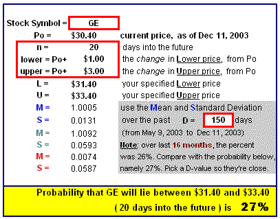

Figure 3

About options: Suppose you're buying a call option with a strike price of $K and you've paid $C for the option, and the option expires in n days, then the stock had better end up at a price bigger than $(K+C) in order to make money. The probability that the stock will be less than $(K+C) is N[log((K+C)/P0), nM, SQRT(n)S)] so the probability that its' greater then $(K+C) is   1 - N[log((K+C)/P0), nM, SQRT(n)S)]   where P0 is today's price. >But it only has to be greater than K+C sometime in the next n days, right? Right, so look at the probability for all values of n less than the number of days to expiry.

Figure 4a

>Okay, what's the probability that the price will be exactly $40?
Zero. However, if we ask for Prob[A < P < B] where B is very close to A, then we'd get (using that Magic Formula):

Prob[A < P < B] = N[log(B/$), nMM, SQRT(n)SS] - N[log(A/$), nMM, SQRT(n)SS] = f[log(A/$), nMM, SQRT(n)SS] log(B/A)     (approximately) where f is the density distribution, as in Figure 4. >The density distribution? Yes, the slope of the cumulative distribution, N. Its maximum occurs at the Mean nMM, so the price is most likely near that value, in n days. However, if you want B = A (hence an exact price), then log(B/A) = log(1) = 0 and ... >Probability = 0, eh? You got it.

Figure 4.

>I have a question.
Shoot.
>Are U and L each Bollinger Bands ... or is it the space between them?
Uh ... I have no idea.