| Standard Deviation ... some thoughts |
When doing the calculations necessary to generate Bollinger Bands one normally ...
>Bollinger?
| Don't you remember? From the above link: | 
|
- Collect stock prices for the past N days: P1, P2, ... PN
- Calculate M, their Mean (or Average) via:
M = (1/N) (P1 + P2 + ... + PN) = (1/N)ΣPm
where Σ means Sum the terms and P1 is the Price N days ago and PN the most recent Price - Calculate SD, the Standard Deviation of this set of Prices via:
Variance = SD2 = (1/N)(P12 + P22 + ... + PN2) - M2(N) = (1/N)ΣPm2 - [(1/N)ΣPm]2
(the average square) minus (the square of the average) ... which is the same as (1/N)Σ(Pm - M)2 - Pick a small number k (example k = 1 or maybe 1.5 or maybe 2) and calculate:
the Upper Bollinger Band via: BU = M + k SD
the Lower Bollinger Band via: BL = M - k SD
|
>So? N = ? k = ?
Patience! In Figure 1, I used N = 20 days and k = 2.0 Standard Deviations. >And the stock price bounces off the Bollinger Bands, eh? That's the idea. To see the geometry more clearly (in this example), we can blow up a part of the chart: 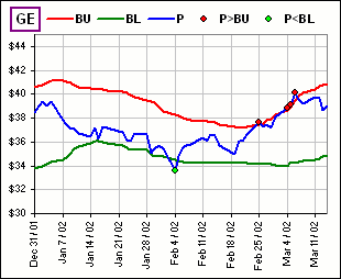 Figure 2 | 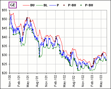 Figure 1 |
|
>Yeah, but isn't that unusual? I mean, the Standard Deviation of Stock Prices? Yes, but it works pretty well, eh? It suggests when to BUY or SELL. However, one normally calculates (and plays with) the Standard Deviation of Stock Returns, not Stock Prices, but ... >Don't tell me! That's the purpose of this tutorial, right?
In what follows. we'll be considering the daily stock Gain Factors rather than stock Returns.
| 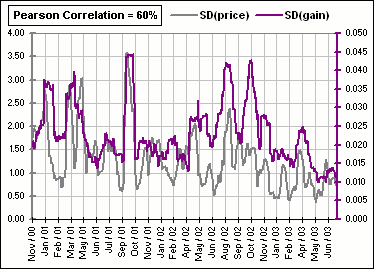 Figure 3 |
Let's suppose that:
- The Stock Price, N+1 days ago, was P0
- Let the daily Gain Factors over the past N days be g1, g2, ... gN
- Let Gm be the cumulative Gain Factor over the first m days, so
Gm = g1g2...gm. - Then the Stock Prices are:
P1 = P0 g1 = P0 G1
P2 = P0 g1g2 = P0 G2
P3 = P0 g1g2g3 = P0 G3
...
PN = P0 g1g2...gN = P0 GN
| If we know the Mean and SD of the gs, what's the Mean and SD of g1 + g1g2 + g1g2g3 + ... +g1g2g3...gm ? |
>Huh? Why is that the question?
Because, whereas the set g1, g2, g3, ... are the daily Stock Gain Factors,
the daily Stock Prices depend upon
g1, g1g2, g1g2g3, ... and we're interested in
determining the relationship between ...
>Yeah, I remember: the relationship between the g's and the G's.
Right, because the G's are products of the g's, like g1g2g3...
We assume we know the parameters for the daily Gain Factors, g1, g2, g3, ...assumed to be random variables:
| Mean(g) = g |
| SD(g) = s |
Okay, now we have the following magic formula:
As noted here:
{
Mean(xy) - Mean(x) Mean(y)
} = SD(x)SD(y) R
where R is the Pearson correlation between the random variables x and y.
We'll assume that our Gain Factors gm are independent, so R = 0 so that
Mean(gigj) = Mean(gi) Mean(gj)
... and that extends to a product with umpteen terms. That is, the Mean of a Product is the Product of the Means.
>The g's are independent? Can you assume that?
Why not? We could incorporate all the cross-correlations but day-to-day gains (usually) have small correlation.
For example, the Pearson correlation between successive daily gains, for the GE example, above, is about -1.6% so it's seems
reasonable (and greatly simplifies the math) ...
>Yeah, yeah. Sounds like a math gimmick to me.
A math gimmick, eh? Yes, analysts always often use such gimmicks, like assuming a Lognormal distribution. It makes life easier.
Anyway, if the g's are uncorrelated, we say that
Mean(g1g2... gm) = Mean(g1) Mean(g2)...Mean(gm)
(where the g's are random numbers selected from some distribution).
Then:
Mean(g1g2... gm) = gm.
Hence, the Mean of N successive Gain Factors = (1/N)[g1 + g1g2 + g1g2g3 + ... + g1g2g3...gN]
= (1/N)[g + g2 + g3 + ... + gN]
and we have a formula for the sum of that series:
| Mean of N successive Gain Factors = Mean(g1 + g1g2 + g1g2g3 + ... + g1g2g3...gN ) = (1/N)[g(gN - 1)/(g - 1)] |
Okay, now on to the Standard Deviation:
For independent random variables x and y, we have another magic formula:
SD2(x*y)
= Mean2(x)SD2(y)
+ Mean2(y)SD2(x)
+ SD2(x)SD2(y)
We can write this as:
[*]
SD2(g1g2...gm-1gm)
=
Mean2(g1g2...gm-1)SD2(gm)
+
Mean2(gm)SD2(g1g2...gm-1)
+
SD2(g1g2...gm-1)SD2(gm)
or
[*]
SD2(g1g2...gm-1gm)
= (g2+s2)
SD2(g1g2...gm-1) +
g2m-2s2
>This looks awfully familiar.
Yes, we did it here, but we'll repeat it just to avoid going back and forth:
Using [*] and proceeding step-by-step, we get:
| Product | Mean2 | SD2 | |
| g1 | g2 | g2+s2 - g2 = s2 | |
| g1g2 | g4 | (g2+s2)2 - g4 | |
| g1g2g3 | g6 | (g2+s2)3 - g6 | |
| ... | ... | ... | |
| g1g2g3...gm | g2m | (g2+s2)m - g2m |
To get the Variance (or SD2) for N cumulative Gain Factors, we could consider adding the variances for each (in the right-most column, above) but ...
>I assume that the variance of a sum is the sum of the variances?
Only for independent random variables, but the terms g1, g1g2, g1g2g3 etc. are NOT independent.
Finally, then, we have:
SD2(g1 + g1g2 + g1g2g3 + ... +g1g2g3...gN)
=
Σ
(g2+s2)j
- Σg2j (j running from j = 1 to j = N)
>And these g1g2 and g1g2g3 ... they're are all independent?
Uh ... not really, but for starters we'll assume that they are.
>Don't you have an "altogether now"?
Note that, when multiplied by the starting Stock Price P0,
the cumulative Gain Factors G1 = g1, G2 = g1g2 etc. are
just the successive daily Stock Prices.
Altogether now:
| [A]
If the daily stock Gain Factors, g1, g2, ... are uncorrelated random variables with Mean(g) = g and SD(g) = s then: |
>You've used a magic formula to add up Σ
(g2+s2)j
- Σg2j ?
Yes.
>I figure there's a lot of hand-waving there. Can you provide some real life ...?
Let's check out the efficacy of these magic formulas, okay?
>Efficacy?
Pay attention.
| 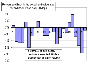 Figure 4 |
|
For a dozen sets of 20-day Stock Prices, we get Figure 4.
>Yeah, so the formula gives a reasonable estimate for the Mean of Stock Prices, but what about GE and what about SD and ... ? Patience, but I should point out that the formula for the SD is ... uh, lousy. Look at Figure 5, for the GE example we started with. It shows, in blue, the actual moving 20-day Average Stock Price and, in red, the Average according to the above formula. That is, we take the Mean daily Gain Factor for the past 20 days (that's g) then we use the formula to estimate the average stock Price, namely: (P0/N)[g(gN - 1)/(g - 1)] >Huh? That's g? What's g?
| 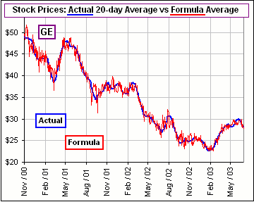 Figure 5 |
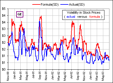 Figure 6 |
>Mamma mia! Something smooth, like the 20-day moving average, turns into ...
Something scary ... which explains why the SD = Volatility formula needs some work >So what does it look like, for the GE example?
Although the Formula Mean stays close to the actual Mean (over 20 days, as in Figure 5), those wee oscillations are pretty wild and they generate a wild and wooly volatility. >But the volatility in Prices is pretty wild too.
|
>So is it always that way or maybe with some other stock or ...
Okay. Consider these:

Figure 7
|
>Aha! Look at the S&P 500! The formula gives a smooother SD!
>And how do Bolli Bands work ... for the S&P? Figure 8 shows the S&P and 20-day, 2-SD Bollinger Bands and ... >Yeah, so why can't you conjur up a formula which generates actual Price volatilities?
>Besides, I thought you wanted to compare two Volatilities: Gains and Prices.
| 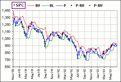 Figure 8 |
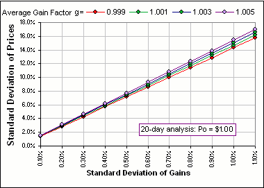 Figure 9 |
Okay, let's assume the Standard Deviation of Gains is s and we stare intently at the formula for the Standard Deviation of
Prices (from [A], above), namely:
SD(Prices) = P0SQRT{[(g2+s2) {(g2+s2)N-1} / (g2+s2-1) - g2 {g2N-1} / (g2-1)]} If we pick a few daily Gain Factors (averaged over 20 days ... that's g) and pick P0 = $1.00 then see how SD(Prices) varies with s... that's SD(Gains) ... we get Figure 9. Remember, g is the average Gain Factor, namely 1+AverageReturn. >It looks linear, eh?
|
>But it doesn't change much with the average daily gain. All the curves are ...
Close together? Yes, so let's analyze.
If we put g = 1+R, where R is the (small) 20-day average daily return, then we can use the fact that,
for small values of x and y,
(1+x)m = 1+mx (approximately) and (1+x)(1+y) = 1+x+y (approximately).
We use these in the magic formula, putting:
- gm = (1+R)m = 1+mR (approximately)
- g2+s2 = 1+2R+s2 (approximately)
- (g2+s2)N = (1+2R+s2)N = 1+2NR+Ns2 (approximately).
SD(Prices) = P0SQRT[ (g2+s2) { (g2+s2)N-1} / (g2+s2-1) - g2 {g2N-1} / (g2-1)]
then becomes:
SD(Prices) = P0SQRT[ (1+2R+s2) (2NR+Ns2)/(2R+s2) - (1+2R)(2NR)/(2R)]
or
SD(Prices) = P0SQRT[N(1+2R+s2) - N(1+2R)]
or
SD(Prices) = P0SQRT[Ns2]
or
SD(Prices) = P0SQRT[N]s = P0SQRT[N]SD(Gains)
so
SD(Prices) / SD(Gains) = P0SQRT[N]
Moral?
We might expect that the Standard Deviation of Prices is a multiple of the Standard Deviation of Gains,
the multiplier being proportional to the square root of N (the number of days, say N = 20) and the initial Price P0
(that'd be 21 days ago).
>I thought we were talking 20 days, not 21.
Uh, you're right. It's 20 days ago, but we're considering a total of 21 days 'cause you need 21 prices to calculate 20 daily gains.
>Aah, I see. And the average daily gain g disappears.
It's not a daily gain, it's a daily gain factor, but yes, in this small-return-approximation it cancels out which explains why the various graphs in Figure 9
are so close together.
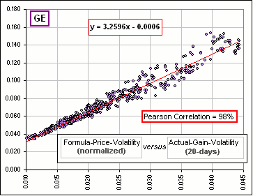 Figure 10 |
>So the volatility of Prices is proportional to the volatility of Gains. Do you believe that?
>And that's it? You've finished?
>I haven't the faintest idea of what Figure 10 is saying!
|
|
>But 98% correlation! Wow!
>But what about the correlation between actual SD(Prices) and actual ...?
>You're comparing formulas for Gain volatilities and Price
volatilities and actual Gain volatilities and Price volatilities. It's confusing!
>zzzZZZ | 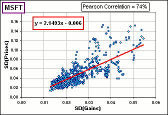 Figure 11 |
Just RIGHT-click and Save Target ... here.
See also this.


