Okay, here's the problem:

• We have a set of n variables, say R₁, R₂, ... R_n   (such as the monthly returns for n stocks).
• The covariance matrix Θ is known   (for these R-variables).
• Construct the linear combination: W = x₁R₁ + x₂R₂ + ... +x_nR_n.
• Choose the weights x_k so as to maximize the Variance of the variable W.

>Huh?
Suppose the R-variables were the stock returns for umpteen stocks, say the stocks in the S&P500, and we wanted to construct a variable which reflects the variations in that collection of stocks.

>Then just use the S&P500 Index, right?
Well, yes ... but many of those 500 stocks are so highly correlated that perhaps we could ignore some.
For example, suppose we took a single stock to represent the entire automobile industry and one to be a proxy for the computer industry and another to ...

>And end up with just 30 instead of 300? You're talkin' the DOW, eh?
Very good!
Let's write our column vectors like so: V = [v₁, v₂, ... ]
I know! It looks like a row vector ... but this notation don't take up so much room.

Then here's the problem, in math-speak:

Given the n x n covariance matrix Θ, determine the n-vector of weights X = [x1, x2, ... xn] such that       XT Θ X = maximum       subject to the constraints: XT X = 1   and   xk ≥ 0   for k = 1, 2, ...n.

>That's the problem? What happened to the R-variables?
As it turns out, the Variance of a portfolio of n assets with covariance matrix Θ is given by:
      σ² = X^T Θ X = Θ₁₁x₁² + Θ₂₂x₂² + ... + Θ_nnx₁² + 2 Θ₁₂ x₁x₂ + 2 Θ₁₃ x₁x₂ + ... etc. etc.

SO, we maximize that Variance. However, we want our weights to be positive and the weight vector X to be of unit length ... hence the constraints.

>And can you solve that problem?
Here's what we know:

• The matrix Θ is symmetric.
• The eigenvalues λ and eigenvectors u satisfy Θ u = λ u.
• Symmetric matrices have real eigenvalues and, if they are all distinct, the eigenvectors are orthogonal.
  That is: if u_j and u_k are two eigenvectors, u_j^Tu_k = 0.
• If that is the case, and we write our X as a linear combination of the unit eigenvectors, X = a₁u₁ + a₂u₂ + ... +a_nu_n, then
  X^T Θ X = {a₁u₁^T + a₂u₂^T +...} Θ {a₁u₁ + a₂u₂ +...} = SUM of terms like: a_ju_j^T Θ a_ku_k
• But Θ u_k = λ_ku_k   (since u_k is an eigenvector)   and u_j^Tu_k = 0   (since eigenvectors are orthogonal).
• Hence:    X^T Θ X = SUM of terms like: a_jλ_ju_j^Tu_j   for j = 1, 2, ... n.
• Since we picked unit eigenvectors, then u_j^Tu_j = 1.
• Further, we required that X^T X = 1, so that Σ a_j² = 1   for j = 1, 2, ... n.

We're almost there!
Clearly we should identify the largest eigenvalue, say λ₁, and choose a₁ = 1 and all other a_j = 0.
That'd make X = u₁ and the weights that'd give the maximum variance are just the components of the eigenvector associated with the largest eigenvalue.

Did you get that?
>zzzZZZ
Don't you see? If X = u₁ (the eigenvector with the largest eigenvalue), then Θ X = Θ u₁ = λ₁u₁ and X^T Θ X = u₁^Tλ₁u₁ = λ₁   ... since u₁^Tu₁ = 1
... and they ain't any bigger eigenvalue than λ₁.

>And just how do you find that eigenvector associated with the largest eigenvalue?
Here's one way to identify the eigenvector of a matrix A associated with the largest eigenvalue:

1. Pick any vector v.
2. Multiply by your matrix A, giving Av.
3. If v = a₁u₁ + a₂u₂ + ..., then Av = a₁λ₁u₁ + a₂λ₂u₂ + ...
4. Repeating umpteen times, we get: A^Nv = a₁λ₁^Nu₁ + a₂λ₂^Nu₂ + ...
5. After each preMultiplication by A, normalize the resultant vector so it's of unit length ... then continue multiplying by A.
6. Eventually, the largest eigenvalue dominates and you're left with a₁λ₁^Nu₁, normalized to unit length- you've identified the appropriate eigenvalue u₁.

>Huh?
Well, for example, suppose and we start with, say v = [1.00, 0.25]
We'll multiply by A, normalize, multiply again ... and again, and we'll see something like this, where v is coloured blue and Av is coloured red, then we normalize A v and it becomes our new v so we colour it blue and the next multiplication (after nomalization) is coloured red again and ...

>Okay! I get it!
Did you see? After just five iterations the vector hardly changes. We've got ourselves the eigenvector u₁.

>But what's that maximum Variance? I thought we ...
Haven't you been listening? The Variance is X^T Θ X which is just λ₁, the largest eigenvalue ... when you choose X = u₁.

>But have you reduced the number of components? I thought you were talking retaining the "principal: components and ...
Patience.
However, notice some things:

1. The coVariance matrix Θ is real and symmetric and is (usually) obtained from historical data.
2. If Θ is n x n, then we can expect n eigenvectors and n associated eigenvalues.
3. The eigenvectors, satisfying Θ u = λ u, have a particular direction, but can be any length.
4. If the n eigenvalues are λ₁, λ₂, ... λ_n, then the contribution to the variance provided by the eigenvector u_k is λ_k / Σλ_j
5. Although one can use the raw historical returns data to calculate Θ, it is better to "normalize" the returns by subtracting the Mean Return then dividing by the Standard Deviation.

>Huh?
If one of the assets has returns r₁, r₂, ... with Mean = m and Standard Deviation = m, then replace the set of returns by (r₁ - m)/s, (r₂ - m)/s ...
That'll change the coVariance matrix into the Correlation matrix ... and that's good because we're only interested in the deviations of returns from their mean, measured as multiples of their Standard Deviation.

>But have you reduced the number of components? I thought ...
If we're willing to accept the allocation identified by the eigenvector u₁, then we've got a single number to represent the Variance provided by the entire set of assets. In other words, if there were 500 stocks and we constructed a single Index composed of a particular allocation of those 500 stocks (defined by u₁), then we've got ourselves a single number, right?

>That's confusing. Do you really understand this stuff?
Want the simple answer? No!
However, I have this spreadsheet that's fun to play with. It looks like this:

Click on picture to download spreadsheet

It'll download 8 years of historical monthly returns for four stocks and construct a coVariance matrix (called A in the spreadsheet).
There's a sheet called Assets which'll do that for you. You can also download (and plot) a "comparison" stock ... like ^DJI.
You then type in some initial 4-vector to start (called V in the spreadsheet) and click a button.
The largest eigenvalue and associated eigenvector are then identified.

>So, in the example, the allocation 30% GE + 28% MSFT + 18% XOM + 24% GM ... does what?
Supposedly, that combination will explain "most" of the Variance of those four stocks ... in a single number.

>And does it?
How would I know?
Anyway, if you're not satsified that the "principal" eigenvector doesn't reflect the collection of stocks, add the next eigenvector, associated with the next largest eigenvalue ... and so on and so on.

>And where are all the other eigenvectors and eigenvalues?
I haven't found them ... yet!
Notes:

The spreadsheet does a bunch of A-multiplications of your initial V, normalizing after each multiplication, until the angle between V and AV is (effectively) 0 degrees. That means that AV and V are in the same direction, so one is a scalar multiple of the other. That is, AV = λV and we've got our eigenvalue/vector pair.

Also, the "Normalized" returns are used for each stock, so the coVariance matrix is really the Correlation matrix.

Having found the "principal" eigenvector and eigenvalue, we'd see if the contribution to our "Index" is large enough.
If not, we look at the next largest eigenvalue and associated eigenvector.

>The next largest? How do you find that?
Since the eigenvectors / eigenvalues satisfy AV = λV, then (A - λI) V = 0, so the matrix A - λI must have a zero determinant.
So, putting det |A - λI | = 0, that gives a polynomial equation to solve for the various eigenvalues λ_k.
The spreadsheet has a plot of this polynomial, somewhere (which, in our case happens to be of 4th order) and ...

>Picture, please! It looks like this   Notice the size of the largest of the four eigenvalues?       >I'd say it was ... uh, 1.7 or thereabouts. It's in the spreadsheet picture above. It's 1.735. In our example, the four eigenvalues are: 0.512, 0.752, 1.001 and 1.735 and their sum is 4.000. So the "weights" associated with the four stocks are: 0.512/ 4.000 = 13%, 0.752/ 4.000 = 19%, 1.001/ 4.000 = 25% and 1.735/ 4.000 = 43%.

>How do I find those other eignevalues? Do I pick them from the chart and ...
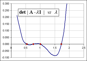You stare at the chart, select four Guesses, then click a button to get better and better estimates.
The spreadsheet will do that, somewhere ... like this.

>Is that 13%+19%+25%+43% good ... or what?
How would I know?
>What do you know?
How would I know?

>Well, at least let's see another example! Okay, here's 8 years worth of four monthly mutual fund returns: VFINX (a 500 Index) VBMFX (Total Bond Index) VIVAX (a Value Fund) VGTSX (International Fund) The eigenvalues, 0.069, 0.235, 0.933 and 2.763, are here >Hey! That largest eigenvalue is really big compared to the others, eh? Yes. As before, we can calculate the contribution to the total Variance as: 2.763 / (0.069+0.235+0.933+2.763) = 2.763 / 4 = 0.69 or 69%.

>I see that the sum of eigenvalues if "4" ... again! What a coincidence!
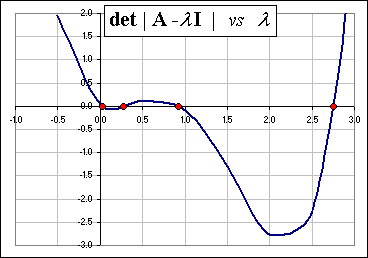Actually, it isn't. It's always the trace of the coVariance matrix = sum of the diagonal elements (which have the value "1") ... so for "4" stocks it'd be "4".

>And the principal eigenvector?
The principal eigenvector is [0.580, -0.191, 0.571, 0.549] which means the allocations should be in these proportions,
and that gives (to the nearest integer):   38%, -13%, 38% and 37%   (adding to 100%) and ...

>Wait a minute! A negative percentage? Are you kidding?
Uh ... well, I understand that sometimes happens so ...

>Sometimes happens! Are you kidding?
The math doesn't know, yet, that the weights have to be positive, so ...
>Then tell it!
Patience.
In the meantime, consider allocating a 4-stock portfolio according to the weights assigned by that principal eigenvector.

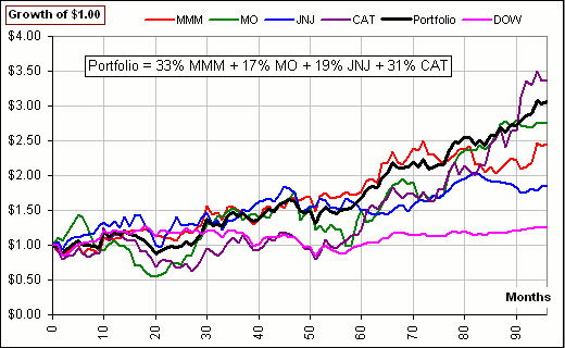
For example, considering the 30 stocks on the DOW, Ron McEwan identified four as being top ranked, according to PCA: MMM, MO, JNJ and CAT. The principal eigenvector (normalized to a unit vector) turned out to be: [0.33, 0.17, 0.19, 0.31]     ... see this A Portfolio of 33% MMM + 17% MO + 19% JNJ + 31% CAT had a chart like so See the Portfolio ... and see the DOW itself? Over the past eight years the Portfolio total return was over 200% while the poor ol' DOW barely managed 26%. Good, eh? >So your portfolio was up 200%? Uh ... hardly.

for Part II

The pictures and spreadsheet may change without noitce