| Ito, Brownian Motion and Black-Scholes ... a summary for Ito-Black-Scholes |
Patient Reader: The route(s) we've taken to explain Ito Math and Brownian Motion and the Black-Scholes option pricing formula are quite tortuous, so here we summarize ...
>Thank God!
Pay attention.
| 1 A Brownian Motion x(t) has the following properties:
 
|
| 2 If x(t) is a Brownian Motion on [0,T], then  x(t) dx(t) = (1/2) [x2(T) - x2(0)] - T/2 x(t) dx(t) = (1/2) [x2(T) - x2(0)] - T/2
|
| 3 If P(x) is a sufficiently well-behaved function of x and x(t) is a Brownian Motion, then dP = P'(x) dx + (1/2) P''(x) dt which follows from a Taylor series expansion of P(x+Δx)-P(x),
using Δx2 = Δt
or dx2 = dt
P(x(T)) - P(x(0))
= where the second integral is Riemann, but the first integral is an Ito integral (because of the stochastic dx). |
| 4 If P(t,x) is a sufficiently well-behaved function of t and x and x(t) is a Brownian Motion, then dP = Pt dt + Px dx + (1/2) Pxx dx2 = [Pt + (1/2) Pxx]dt + Px dx
which follows from a Taylor series expansion of P(t+Δt, x+Δx)-P(t,x), using Δx2 = Δt or dx2 = dt |
| 5 [Ito's Lemma] If P(t,x) follows a stochastic process, described by dP = μ(t,P)dt + σ(t,P)dx and x(t) is a Brownian Motion (so, among other things, dx2 = dt) then F(t,P), any sufficiently smooth function of t and P, satisfies: dF = Ft dt + FP dP + (1/2) FPP dP2 = [FPμ + Ft + (1/2)FPPσ2]dt + FPσdx (substituting for dP) |
| 6 If r is the Mean Return and s is the Standard Deviation, then we assume that changes in stock Price satisfy: dP = r P dt + s P dx, a Geometric Brownian Process. This has solution: P(t) = P(t0) exp[(r-s2/2)(t-t0) + s (x(t)-x(t0))] where x(t) is a Brownian Motion with a Normal density distribution described by: G(u) = 1/SQRT[2πT] EXP[- u2/2T] with T = t - t0. meaning that the probability that X(t) = x(t) - x(t0) lies in [u,u+du] is G(u) du.  
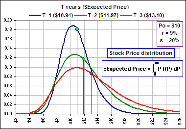
Typical Price charts (with a Brownian component B(t)) The Price, as given above, will generate the distribution:
|
Two reminders: Normal and Lognormal distributions:
| 7 [Normal] If f(x) is a normal density distribution for X, with Mean = m, Standard Deviation = S, then 
meaning: the probability that X lies in [x,x+dx] is f(x)dx. | 
|
| 8 [Lognormal] The (lognormal) distribution of Prices P at time T = t - t0, if P(t0) = Po, is  note: log is the natural logarithm note: log is the natural logarithm
meaning: the probability that the Price lies in [P,P+dP] is f(P)dP. Note: The Expected value of P(T) is E[P(T)] = Po erT | 
|
Now on to Option pricing ...
| 9
Consider a call option with value C(t,P), depending upon the stock price P satisfying 6, and we have (see 4): dC = Ct dt + CP dP + (1/2) CPP s2P2dt Substituting for dP gives: dC = [rPCP + Ct + (1/2)s2P2CPP]dt + sPCPdx ... which we'll call AC dt + BC dx. where A C = [CPrP + Ct + (1/2)CPPs2P2] and B C = CPsP |
| 10
Selecting a Portfolio made up of stock (price=P) and options on that stock (price=C) and $Q in a risk-free asset with return R, we devote fractions u, v and w=1-u-v to each asset and get: d(Portfolio) / Portfolio = [su + Bv] dx + [ru + Av + Rw] dt Now choose u and v, the fractions devoted to stocks and options, so that su + Bv = 0 (eliminating the Portfolio randomness associated with the dx) and E[d(Portfolio) / Portfolio] = [ru + Av + Rw] dt = R dt meaning our Portfolio is expected to grow at the risk-free rate R. This gives the Black-Scholes-Merton equations: from which (eliminating u and v) we get: (r-R)/s = (A-R)/B ... giving [!!] AC = RC + BC(r-R)/S so the Sharpe Ratio for the option should be the same as for the stock (for our riskless Portfolio) and we now expect our Portfolio to generate the risk-free return R. Substituting for A and B (from 9 into [!!]) gives rise to an non-stochastic PDE for C, namely: |
| 11 [Black-Scholes] The Black-Scholes partial differential equation for C(t,P), the option premium, is: Ct + R P CP+ (1/2)s2P2 CPP = R C with the underlying stock price P a Geometric Brownian Process satisfying dP = (r dt+ s dx)P, x(t) being a Brownian Motion and R is a risk-free rate. |
| 12 If the strike price of the option is K then, at maturity (after a time T = t-t0), it's worth Max(P - K,0). Discounting at the risk-free rate R, it's Expected value today is then exp(- RT)E[Max(P-K,0)]. To compute this Expected value, we use distribution of stock prices at maturity, f(P), and get: C = exp(- RT)[  P f(P) dP - K P f(P) dP - K f(P) dP] f(P) dP]
Using f(P) from 6, we get the Black-Scholes option premium 
|

The Black-Scholes Option Pricing Formula |
>zzzzz
How about some pictures?


|
Do you recognize lognormal when you see it?
|
Do you see that, above the strike price, the call premium increases almost linearly with the current stock price? That's because d1 and d2 are large enough to make N(d1) and N(d2) nearly "1" so C = P(0)N(d1) - K e-RTN(d2) is nearly C = P(0) - K e-RT and since RT is near 0 (example: RT = 0.09*0.75 = 0.068) so e-RT is nearly 1 (example: e-0.068 = 0.93) so, very nearly, C = P(0) - K and that's the equation of the almost straight line in the lower chart above and ... >zzzZZZ | 
|
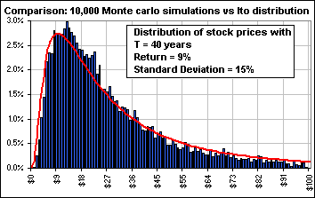
In order to check that magic prescription for the stock price distribution, T = 40 years in the future,
I did a bunch of Monte Carlo simulations (choosing random annual returns from a lognormal distribution with:
Mean Return r = 9% and Standard Deviation s = 15% and initial price Po = $1.00
in order to see how well that formula fit the Monte Carlo result. Here's what I got:
the Ito formula
| 
|
>zzzZZZ
Okay, let's call it a day.
References go here: (when I get all the URLs straightened out :^)
Loren Cobb Ito and Black-Scholes.pdf Shreve: Stochastic Calculus Black-Scholes Equation Random Walks in Physics.pdf
You can also play with this online spreadsheet: Click!

